


Download NCERT Class 11 Maths Solutions PDF
NCERT Solutions for Class 11 Maths provide detailed and systematic explanations for all the chapters in the CBSE syllabus for the 2026-27 academic year. These solutions simplify complex problems and help students understand key concepts in topics like Quadratic Equations, Statistics, and Trigonometry. With clear, step-by-step solutions, students can easily grasp difficult topics and improve their problem-solving skills. The NCERT Maths solutions are designed to clear doubts and enhance your mathematical skills. These solutions include sample-solved questions, shortcuts, and summaries, making your study sessions more efficient. For easy access, you can download the solutions in PDF format and study them offline. Simply click on the “Download PDF” button at the top of each chapter page to access the materials.
 Table of Content
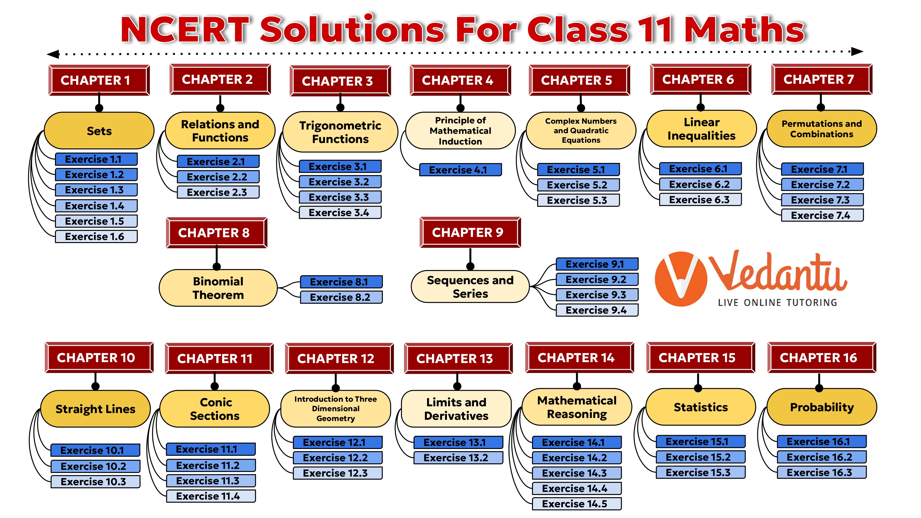
NCERT Solutions for Class 11 Maths- FREE PDF Download
Note: The chapters on Principle of Mathematical Induction and Mathematical Reasoning have been excluded from the Class 10 Maths textbook for the 2026-27 academic year
Also check for: What are the important topics covered in the NCERT Solutions Class 11 Maths?

FAQs on NCERT Solutions For Class 11 Maths - 2026-27
1. Are Vedantu’s NCERT Solutions enough for Class 11 Maths exam preparation?
Yes, the NCERT textbook and these step-by-step solutions are sufficient for CBSE exams. They build a strong foundation, clarify concepts, and match the types of questions asked in the final exam. For extra practice, you may also solve NCERT Exemplar problems.
2. How do Class 11 Maths NCERT Solutions help improve exam scores?
These solutions provide detailed, CBSE-aligned methods for every problem, helping you understand the correct approach, improve accuracy, and manage time better in exams.
3. Are the NCERT textbook and its solutions sufficient for the Class 11 Maths final exam?
Yes, the NCERT textbook is the most important book as the final exam paper is primarily based on its syllabus and exercise questions. Using the corresponding NCERT Solutions ensures you master the core concepts and question patterns. For advanced preparation and to tackle higher-order thinking skill (HOTS) questions, students can also refer to the NCERT Exemplar.
4. Which chapters in Class 11 Maths hold the most weightage in the final exam?
According to the CBSE exam pattern for 2026-27, the marks are distributed across units. The units with significant weightage are:
- Sets and Functions: Covers fundamental concepts and carries high importance.
- Algebra: Includes topics like Complex Numbers, Linear Inequalities, and Sequences and Series.
- Coordinate Geometry: Focuses on Straight Lines and Conic Sections.
- Calculus: Introduces Limits and Derivatives, a crucial unit for Class 12.
5. What is an effective strategy to use these NCERT Solutions for exam preparation?
For the best results, first attempt to solve the exercise questions on your own. Then, use the NCERT Solutions to:
- Verify your answers and check the methodology.
- Understand the step-wise marking scheme followed by CBSE.
- Identify and learn from your mistakes.
- Discover more efficient or alternative methods to solve a problem.
6. Which topics in Class 11 Maths are generally considered the most challenging?
While difficulty is subjective, students often find the following chapters more demanding due to their abstract nature and complex problem-solving techniques:
- Trigonometric Functions: Involves numerous identities and graphs.
- Permutations and Combinations: Requires strong logical reasoning.
- Conic Sections: Involves detailed geometric derivations.
- Limits and Derivatives: A foundational but conceptually new topic in calculus.
7. What is the difference between NCERT textbook exercises and NCERT Exemplar problems?
NCERT textbook exercises are designed to build a strong fundamental understanding of concepts and cover the core syllabus. NCERT Exemplar problems, on the other hand, are of a higher difficulty level. they are designed to test in-depth knowledge, application skills, and prepare students for more challenging questions, including those in competitive exams.
8. How can using NCERT Solutions improve problem-solving speed and accuracy?
Consistent practice with NCERT Solutions helps you internalise the most efficient problem-solving methods. By repeatedly reviewing the correct step-by-step procedures, you reduce the chances of making calculation or methodological errors. This familiarity builds confidence and allows you to solve problems faster and more accurately during exams.