Probability Class 12 Notes: CBSE Maths Chapter 13

Basic Definitions:

Random Experiment:

• An experiment in which all possible outcomes are known ahead of time, but the outcome of any particular performance cannot be predicted until the experiment is completed.

• For example - Tossing of a coin, throwing a dice, etc.

Sample-space:

• A collection of all conceivable outcomes from a single random experiment.

• Sample space is denoted as ‘$$S$$’.

• For example:  If we're interested in the number that appears on the top face of a die, sample space would be 

$$S=\{1,2,3,4,5,6\}$$

Experiment or Trial:

• It is a succession of actions with unpredictably unclear outcomes.

• Example - Tossing of a coin, selecting a card from deck of cards, throwing a dice.

Event:

• Subset of sample – space.

• In any sample space, we might be more interested in the occurrence of various occurrences than the existence of a given element.

Simple Event:

• If an event is a set with only one sample-space element, it is called a single-element event.

Compound Event:

• A compound event can be represented as a collection of sample points.

• Example:

Event of drawing a spade from a deck of cards is the subset $$A=\left\{\text{spade}\right\}$$ of the sample space $$S=\left\{\text{heart, spade, club, diamond}\right\}.$$

Therefore $$A$$ is a simple event. None the event B of drawing a black card is a compound event since

$$B=\left\{spadeUc\mathrm{lub}\right\}=\{spade,c\mathrm{lub}\}$$.

Probability:

• If each one of $$N$$ alternative equally likely outcomes can result from a random experiment, and if exactly $$n$$ of these events favours $$A$$.

$$A,P\left(A\right)={\displaystyle \frac{n}{N}}$$

That is $${\displaystyle \frac{\text{Favourable Cases}}{\text{Total No}\text{. of Caes}}}$$

• Remarks: 

• Just because a given event has a probability of one does not indicate it will happen with certainty.

• It is just predicting that the event is most likely to occur in contrast to other events. 

• Predictions are based on historical data and, of course, the method of analysing the data at hand.

• Similarly, just because the probability of an occurrence is zero does not mean that it will never happen!

Mutually Exclusive Event:

Two mutually exclusive occurrences cannot occur at the same time.

Independent Events:

When the occurrence or non-occurrence of one event has no bearing on the occurrence or non-occurrence of another, the events are said to be independent.

Exhaustive Event:

If a random experiment always results in the occurrence of at least one of a set of events, it is said to be exhaustive.

Conditional Probability:

• The conditional probability is the probability that an event $$B$$ will occur given the knowledge that an event $$A$$has previously occurred.

• This probability is written $$P\left(B|A\right),$$ notation for the probability of $$B$$ given $$A$$.

• When events $$A$$ and $$B$$ are the independent, the conditional probability of event $$B$$ for event $$A$$ is the probability of event $$B$$, that is $$P$$, in the case when events $$A$$ and $$B$$ are independent (that is, event $$A$$ has no effect on the probability of event $$B$$) $$P\left(B\right)$$.

• Since the events $$A$$ and $$B$$ are not independent, the probability that they will intersect (that both events will occur) is given by

$$P\left(A\text{ and }B\right)=P\left(A\right)P\left(B|A\right)$$.

• If a random experiment has two sample space of $$E$$ and $$S$$ that these two events linked with the same sample space, the conditional probability of the event $$E$$ given that $$S$$ has occurred,
  That is, 

$$P(E|S)$$ is given by 

$P(E|S)={\displaystyle \frac{P(E\cap S)}{P(S)}}$ 

Provided  $P(S)\ne 0$ 

• Example:

If $\text{P(A) = }{\displaystyle \frac{5}{\text{12}}}\text{, P(D) = }{\displaystyle \frac{7}{\text{12}}}$ and $P(A\cap D)={\displaystyle \frac{3}{12}}$ , evaluate $$P(A|D)$$.

$$P(A|D)={\displaystyle \frac{P(A\cap D)}{P(D)}}$$

$$P(A|D)={\displaystyle \frac{{\displaystyle \frac{3}{12}}}{{\displaystyle \frac{7}{12}}}}$$

$$P(A|D)={\displaystyle \frac{3}{7}}$$

Properties of Conditional Probability:

Let’s consider $$E$$ and $$F$$ be the events of a sample space $$S$$ of an experiment, then

Property $$1$$ :

$$P\left(S|F\right)=P\left(F|F\right)=1$$ 

We know that,

$$P(E|F)={\displaystyle \frac{P(S\cap F)}{P(F)}}={\displaystyle \frac{P(F)}{P(F)}}=1$$

Also,

$$P(F|F)={\displaystyle \frac{P(F\cap F)}{P(F)}}={\displaystyle \frac{P(F)}{P(F)}}=1$$

Thus,

$P(S|F)=P(F|F)=1$ 

Property $$2$$:

Let’s consider that $$M$$ and $$N$$be the any two events of a sample space $$S$$ and $$F$$ be an event of $$S$$ such that$$P\left(F\right)\ne 0$$ , then

$P((M\cup N)|F=P(M|F)+P(N|F)-P((M\cap N)|F$ 

If $$M$$and $$N$$ are discontinuous events,

$P((M\cup N)|F)=P(M|F)+P(N|F)$

We have 

$P((M\cup N)|F)={\displaystyle \frac{P[(M\cap N)|F]}{P(F)}}$

$={\displaystyle \frac{P[(M\cap F)\cup (N\cap F)]}{P(F)}}$

(Based on the distributive law of set union over intersection)

$={\displaystyle \frac{P(M\cap F)+P(N\cap F)-P(M\cap N\cap F)}{P(F)}}$

$$={\displaystyle \frac{P(M\cap F)}{P(F)}}+{\displaystyle \frac{P(N\cap F)}{P(F)}}-{\displaystyle \frac{P[(M\cap N)\cap F]}{P(F)}}$$ 

$=P(M|F)+P(N|F)-P((M\cap N)|F)$ 

When $$N$$ and $$N$$ are disjoint events, then

$P((M\cap N)|F)=0$

$\Rightarrow P((M\cup N)|F)=P(M|F)+P(N|F)$

Property $$3$$ :

$P(E^{\prime }|F)=1-P(E|F)$ 

From Property 1, 

$P(S|F)=1$ 

$\Rightarrow P(E\cup E^{\prime }|F)=1$ Since, $S=E\cup E^{\prime }$ 

$\Rightarrow P(E|F)+P(E^{\prime }|F)=1$ Since, $E$ and $E^{\prime }$ are disjoint events

Thus, 

$P(E^{\prime }|F)=1-P(E|F)$

Multiplication Theorem on Probability:

• Let $$E$$ and $$F$$ be two events linked with a sample space $$S$$.

• $$P\left(E|F\right)$$ denotes the conditional probability of event $$E$$ given that $$F$$ has occurred .

$P(E|F)={\displaystyle \frac{P(E\cap F)}{P(F)}},P(F)\ne 0$ 

• From this result, we can write

$P(E\cap F)=P(F).P(E|F)........(1)$ 

Also, we know that

$P(F|E)={\displaystyle \frac{P(F\cap E)}{P(E)}},P(E)\ne 0$

or $P(F|E)={\displaystyle \frac{P(F\cap E)}{P(E)}}$ (since $E\cap F=F\cap E)$ 

Thus, $P(E\cap F)=P(E).P(F|E).........(2)$ 

Combining (1) and (2), we find that

$P(E\cap F)=P(E).P(F|E)$

$=P(F).P(E|F)$ 

Since, $P(E)\ne 0$ and $P(F)\ne 0$.
The above result is called as the Multiplication rule of probability.

• Example:

There are $$25$$ black and $$30$$ white balls in an urn. Two balls are drawn one after the other from the urn without being replaced. Is it likely that both drawn balls will be black?

Ans.:

Consider, $$E$$ and $$F$$ are representing the events in which the first and second balls drawn are both black.

$$P\left(E\right)=P$$ (Black ball in first draw) $={\displaystyle \frac{25}{55}}$ 

Given that the first ball chosen is black, the event has taken place, and the urn now contains both $$24$$ black and $$30$$ white balls.

As a result, the conditional probability of  $$F$$ given that $$E$$ has occurred is the given that the first ball pulled was black, the likelihood of the second ball being black is high.

That is

$$P\left(F|E\right)={\displaystyle \frac{24}{54}}$$

By multiplication rule of probability, we have

\[P\text{ }\left( E\text{ }\cap \text{ }F \right)\text{ }=\text{ }P\text{ }\left( E

\right)\text{ }P\text{ }\left( F|E \right)\] 

$$={\displaystyle \frac{25}{55}}\times {\displaystyle \frac{24}{55}}={\displaystyle \frac{600}{3025}}$$ 

$$={\displaystyle \frac{24}{121}}$$

Note:

• Probability multiplication rule for more than two events if  $$E$$ is true, $$F$$and $$G$$ are three events of sample space, we have

$$P(E\cap F\cap G)=P\left(E\right)P\left(F|E\right)P\left(G|(E\cap F)\right)=P\left(E\right)P\left(F|E\right)P\left(G|EF\right)$$ 

• Similarly, the probability multiplication rule can be extended to four or more events.

Independent Events:

• If $$E$$ and $$F$$ are two events whose likelihood of occurrence is unaffected by the probability of occurrence of the other. Independent events are what they're termed when they happen on their own.

• If $$E$$ and $$F$$ are two events that occur during the same random experiment, they are considered to be independent.

$$P(E\cap F)=P\left(E\right).P\left(F\right)$$ 

Remarks:

• Two events $$E$$ and $$F$$are dependent if they are not independent, that is 

$$P(E\cap F)\ne P\left(E\right).P\left(F\right)$$ 

• It's easy to get mixed up between independent and mutually exclusive events.

• The term "independent" is defined in terms of "event probability," whereas "mutually exclusive" is defined in terms of "event probability" (subset of sample space).

• Mutually exclusive events will never have a shared result, whereas independent events may.

• Two mutually exclusive events with nonzero possibilities of occurrence cannot be mutually exclusive, and two mutually exclusive occurrences with nonzero probabilities of occurrence cannot be mutually exclusive.

• Two experiments are independent for every pair of events $$E$$ and $$F$$, where first experiment is linked with the second experiment, then the probability of the simultaneous occurrence of the events $$E$$ and $$F$$only when the two experiments are performed which is the product of $$P\left(E\right)$$ and $$P\left(F\right)$$ calculated separately on the basis of two experiments, that is 

$$P(E\cap F)=P\left(E\right).P\left(F\right)$$ 

• Three events $$A,B$$ and $$C$$ are said to be mutually independent, if

$$P(A\cap B)=P\left(A\right)P\left(B\right)$$ 

$$P(A\cap C)=P\left(A\right)P\left(C\right)$$ 

$$P(B\cap C)=P\left(B\right)P\left(C\right)$$ and

$$P(A\cap B\cap C)=P\left(A\right)P\left(B\right)P\left(C\right)$$ 

We argue that three occurrences are not independent if at least one of the aforementioned conditions is not met.

• Example

A die is thrown. Let $$E$$ be the event ‘the number appearing is a multiple of $$2$$  and $$F$$ be the event ‘the number appearing is odd’ then find whether $$E$$ and $$F$$ are independent?

Solution:

The sample space is $$S=\{1,2,3,4,5,6\}$$ 

Now $$E=\{2,4,6\},F=\{1,3,5\}$$ and $$E\cap F=\left\{4\right\}$$ 

Then

$$P\left(E\right)={\displaystyle \frac{3}{6}}={\displaystyle \frac{1}{2}}$$ 

$$P\left(F\right)={\displaystyle \frac{3}{6}}={\displaystyle \frac{1}{2}}$$ 

$$P(E\cap F)={\displaystyle \frac{1}{4}}$$ 

Clearly,

$$P(E\cap F)=P\left(E\right).P\left(F\right).$$ 

Hence, $$E$$ and $$F$$ are independent events.

Bayes' Theorem: Description:

• Also called as inverse probability theorem

• Consider that there are two sacs $$I$$ and $$II$$ .

• Sac $$I$$ contains $$2$$  white and $$3$$  red kites

• Sac $$II$$ contains $$4$$  white and $$5$$  red kites.

• One kite is drawn at random from one of the sacs.

• Probability of selecting any of the sac (that is ${\displaystyle \frac{1}{2}}$) or probability of drawing a kite of a particular colour that is white from a particular sac $$I$$.

• If we are given the sac from which the kite is drawn, the probability that the kite drawn will be of a specific colour.

• If the colour of the kite pulled is known, we must find the reverse likelihood of sac $$II$$ being selected when an event occurs after it is known to find the probability that the sac drawn is from a particular sac $$II$$.

• John Bayes, a famous mathematician, used conditional probability to address the challenge of obtaining reverse probability.

• As a result, the ‘Bayes theorem' was named after him, and it was published posthumously in $$1763$$.

Definitions:

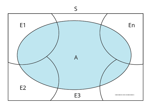
Partition of a sample space:

• The partition of the sample space $$S$$ stated to be a set of events $$E_1,E_2,...,E_n$$

If

• $$Ei\cap Ej=\phi$$ , $$i\ne j,i,j=1,2,3,...,n$$ 

• $$E_1\cup E_2\cup ...\cup E_n=S$$ and

• $$P\left(Ei\right)>0$$ for all $$i=1,2,......,n$$ .

• If the events $$E_1,E_2,...,E_n$$ are pairwise disjoint, exhaustive, and have nonzero probabilities, they represent a partition of the sample space $$S$$.

Theorem of Total Probability:

• Let {$$E_1,E_2,...,E_n$$} be a partition of the sample space $$S$$,

• Suppose that each of the events $$E_1,E_2,...,E_n$$has nonzero probability of occurrence.

• Let $$A$$ be the any event linked with $$S$$, then
  $P(A)=P(E_1)P(A|E_1)+P(E_2)P(A|E_2)......+P(E_n)P(A|E_n)$ 

$=\sum _{j=1}^{n}P(E_j)P(A|E_f)$ 

Proof:

We have given that $$E_1,E_2,...,E_n$$is a partition of the sample space $$S$$. Therefore,

$S=E_1\cup E_2\cup ....\cup E_n$ 

And 

$E_i\cap E_j=\mathrm{\Phi },i\ne j,i,j=1,2,......,n$ 

Now, we know that for any event $A$ ,

$A=A\cap S$ 

$=A\cap (E_1\cup E_2\cup ....\cup E_n)$ 

$=(A\cap E_1)\cup (A\cap E_2)\cup ....\cup (A\cap E_n)$ 

Also $A\cap E_i$ and $A\cap E_j$ are respectively the subsets of $E_i$ and $E_j$. We know that $E_i$ and $E_j$are disjoint, for $i\ne j$ , therefore, $A\cap E_i$ and $A\cap E_j$are also disjoint for all $i\ne j,i,j=1,2,......,n$.

Thus , 

$P(A)=P[(A\cap E_1)\cup (A\cap E_2)\cup ....\cup (A\cap E_n)$

$=P(A\cap E_1)+(A\cap E_2)+....+(A\cap E_n)$             

Now, by multiplication rule of probability, we get

$P(A\cap E_i)=P(E_i)P(A|E_i)$ as $P(E_i)\ne 0\mathrm{\forall }i=1,2,....,n$ 

Therefore, 

$P(A)=P(E_1)P(A|E_1)+P(E_2)P(A|E_2)+.....+P(E_n)P(A|E_n)$ 

Or 

$P(A)=\sum _{j=1}^{n}P(E_f)P(A|E_f)$ 

Bayes' Theorem: Proof:

If $$E_1,E_2,...,E_n$$are n non empty events that make up a partition of sample space S, i.e. $$E_1,E_2,...,E_n$$are pairwise disjoint and $$E_1\cup E_2\cup ...\cup E_n=S$$ and $$A$$ is any event with a probability greater than zero, then

$P(E_I|A)={\displaystyle \frac{P(E_J)P(A|E_i)}{\sum _{j=1}^{n}P(E_J)P(A|E_j)}}$ for any $i=1,2,3,....,n$ 

Proof:

We can conclude from the conditional probability formula that

$P(E_i|A)={\displaystyle \frac{P(A\cap E_i)}{P(A)}}$ 

$={\displaystyle \frac{P(E_i)P(A|E_i)}{P(A)}}$ (By the probability multiplication rule)

$={\displaystyle \frac{P(E_i)P(A|E_i)}{\sum _{j=1}^{n}P(E_j)P(A|E_j)}}$ (As a result of the total probability theorem)

Remark:

When Bayes' theorem is employed, the following nomenclature is commonly used.

• Hypotheses are occurrences such as $$E_1,E_2,...,E_n$$.

• The priori probability of the hypothesis $$Ei$$ is $$P\left(Ei\right)$$.

• The posteriori probability of the hypothesis $$Ei$$ is the conditional probability $$P\left(Ei|A\right)$$.

• The formula for the likelihood of "causes" is also known as the "causes formula." Because the $$Ei$$'s are a subset of the sample space $$S$$, only one of the $$Ei$$'s happens (that is one of the events $$Ei$$ must occur and only one can occur). As a result, provided that event $$A$$ has occurred, the foregoing formula provides us the likelihood of a specific $$Ei$$.

Random Variables and its Probability Distributions:

• As illustrated in the following examples/experiments, we were not only interested in the specific outcome that occurred in most random experiments in Sample space, but also in the number connected with that outcome.

• Experiments:

• While tossing two dice, we can be interested in the sum of the numbers on the two dice.

• We might want to know how many heads we got by tossing a coin $10$ times

• In the experiment of randomly selecting four articles (one after the other) from a batch of $$30$$ articles, $$15$$ of which are defective, we want to know the number of defectives in the sample of four, not in the precise sequence of defective and non-defective products.

• In all of the aforementioned experiments,

• We have a rule that allocates a single real number to each experiment's conclusion. 

• This single real number may change depending on the experiment's outcome. As a result, it is a variable.

• Its value is also determined by the outcome of a random experiment, which is why it is referred to as a random variable.

• $$X$$ is commonly used to represent a random variable.

• Because a random variable can have any real value, the set of real numbers is its co-domain. As a result, a random variable is defined as follows:

• The sample space of a random experiment is the domain of a random variable, which is a real-valued function.

• For instance, consider the experiment of tossing a coin thrice in a row.

• Sample space of the experiment is $$S=\{HH,HT,TH,TT\}.$$ 

• If $$X$$ signifies the number of heads obtained, then $$X$$ is a random variable with the following values for each outcome:

$$X\left(HH\right)=2,X\left(HT\right)=1$$ , $$X\left(TH\right)=1,X\left(TT\right)=0$$ 

• Let $$Y$$ denote the number of heads minus the number of tails for each outcome of the above sample space $$S$$.

• For each outcome of the above sample space $$S$$, let $$Y$$ signify the number of heads minus the number of tails.

• $$Y\left(HH\right)=2,Y\left(HT\right)=0$$ ,$$Y\left(TH\right)=0,Y\left(TT\right)=2$$.

• As a result, $$X$$ and $$Y$$ are two separate random variables defined on the same sample space $$S$$ .

• Note: On the same sample space, many random variables can be defined.

A Random Variable's Probability Distribution:

• The probability distribution of the random variable $$X$$ is a description that offers the random variable's values as well as the probabilities associated with it.

• In general, a random variable's probability distribution is defined as follows:

• The system of numbers is the probability distribution of a random variable $$X$$.

$X:x_1{x}_2.......x_n$ 

$P(X):P_1{P}_2.......P_n$

where,  

$p_i>0,\sum _{i=1}^n{p}_i=1,i=1,2,......,n$ 

The real numbers $x_1,x_2,....,x_n$ are the possible vales of the random variable $X$ and $p_i(i=1,2,...,n)$is the probability of the random variable $X$taking the value $x_i$ that is, 

$P(X=x_i)=p_i$ 

• All elements of the sample space are also covered for all potential values of the random variable $$X$$.

As a result, the total probability in a probability distribution must equal one.

• Only at certain points ($$s$$) in the sample space is $$X=x_i$$ true.

As a result, the probability that $$X$$ takes the value $$x_i$$ is never $$0$$ , that is

$$P(X=xi)\ne 0$$.

Mean of a Random Variable:

• In the sense that it roughly locates the random variable's middle or average value, the mean is a measure of central tendency.

• Consider $$X$$ be a random variable with the possible values $$x_1,{\text{x}}_2,{\text{x}}_3,...,{\text{x}}_n$$occuring with probabilities $$p_1,p_2,p_3,...,p_n$$ , respectively. 

• The mean of $$X$$, denoted by$$\mu$$, is the number$\sum _{i=1}^n{x}_i{p}_i$ that is the mean of $$X$$ is the weighted average of the possible values of $$X$$, each value being weighted by its probability with which it occurs.

• The mean of $$X$$ , represented by $$\mu$$ , is the number $\sum _{i=1}^n{x}_i{p}_i$ that is the mean of $$X$$ is the weighted average of the possible values of $$X$$ , with each value being weighted by its probability of occurrence.

• The expectation of $$X$$ is also known as it’s mean and it’s denoted by $$E\left(X\right)$$.
  Thus,

$E(X)=\mu

=\sum\limits_{i=1}^{n}{{{x}_{i}}{{p}_{i}}}={{x}_{1}}{{p}_{1}}+{{x}_{2}}{{p}_{2}}+....+{{x}_{n}}{{p}_{n}}$ 

• The sum of all possible values of by their respective probabilities is the mean or expectation of a random variable $$X$$ .

Variance of a Random Variable:

• The mean of a random variable provides no information regarding the variability of the random variable's values.

• If the variance is small, the random variable's values are near to the mean. 

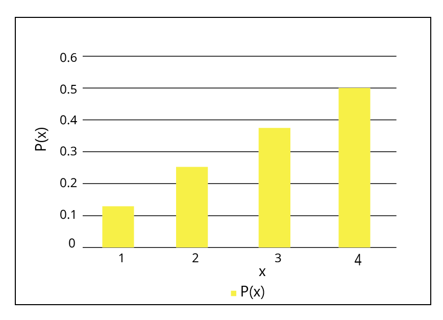
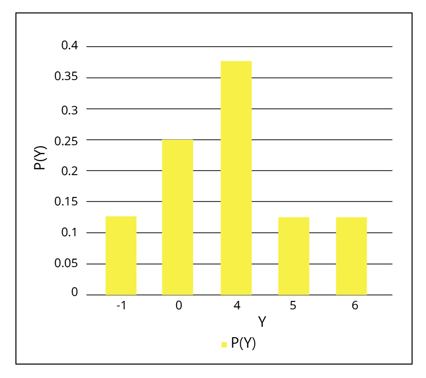
• Random variables with different probability distributions, as demonstrated in the distributions of $$X$$ and $$Y$$ , can have equal means, as illustrated in the following distributions.

$E(X)=1\times {\displaystyle \frac{1}{8}}+2\times {\displaystyle \frac{2}{8}}+3\times {\displaystyle \frac{3}{8}}+4\times {\displaystyle \frac{2}{8}}$ 

$E(X)={\displaystyle \frac{22}{8}}=2.75$

$E(Y)=-1\times {\displaystyle \frac{1}{8}}+0\times {\displaystyle \frac{2}{8}}+4\times {\displaystyle \frac{3}{8}}+5\times {\displaystyle \frac{1}{8}}+6\times {\displaystyle \frac{1}{8}}$

$E(Y)={\displaystyle \frac{22}{8}}=2.75$

Although the variables $$X$$ and $$Y$$ are distinct, their means are the same.

Below is a diagrammatic representation of these distributions.

• Assume that $$X$$ is a random variable with possible values $$x_1,x_2,...,x_n$$ and possible probabilities $$p(x_1),p\left(x_2\right),...,p\left(x_n\right)$$ respectively.

Let $\mu =E(X)$ be the mean of $$X$$. 

The variance of $$X$$, denoted by $Var(X)$ or ${\sigma }_x^2$ is defined as

${\sigma }_x^2=Var(X)=\sum _{i=1}^n{(x_i-\mu )}^{2}p(x_i)$

${\sigma }_x^2=E{(X-\mu )}^2$

or equivalently

${\sigma }_x^2=\sqrt{Var(X)}=\sqrt{\sum _{i=1}^n{(x_i-\mu )}^{2}p(x_i)}$

The non- negative number is known as the standard deviation of the random variable.

The variance of a random variable can be calculated as;

We know that,

$Var(X)=\sum _{i=1}^n{(x_i-\mu )}^{2}p(x_i)$ 

$=\sum _{i=1}^n({x_i}^2+{\mu }^2-2\mu x_i)p(x_i)$

$=\sum _{i=1}^n{x_i}^{2}p(x_i)+\sum _{i=1}^n{\mu }^{2}p(x_i)-\sum _{i=1}^{n}2\mu x_{i}p(x_i)$

$=\sum _{i=1}^n{x_i}^{2}p(x_i)+{\mu }^2\sum _{i=1}^{n}p(x_i)-2\mu \sum _{i=1}^n{x}_{i}p(x_i)$

$=\sum _{i=1}^n{x_i}^{2}p(x_i)+{\mu }^2-2\mu$$[\text{since }\sum _{i=1}^{n}p(x_i)=1\text{ and }\mu =\sum _{i=1}^n{x}_{i}p(x_i)]$ 

$=\sum _{i=1}^n{x}_i^{2}p(x_i)-{\mu }^2$
or 

$Var(X)=\sum _{i=1}^n{x_i}^{2}p(x_i)-{\left(\sum _{i=1}^n{x}_{i}p(x_i)\right)}^2$

or 

$Var(X)=E(X^2)-{[E(X)]}^2$ 

Where,

$E(X^2)=\sum _{i=1}^n{x_i}^{2}p(x_i)$ 

The Binomial Distribution:

• The binomial expansion of the probability distribution of the number of successes in an experiment consisting of  $$n$$ Bernoulli trials may be used to derive the probability distribution of the number of successes in an experiment consisting of $$n$$ Bernoulli trials $${(q+p)}^n$$.

• As a result, this distribution of success numbers $$X$$ can be represented as

• The above probability distribution is known as a binomial distribution with parameters $$n$$ and  $$p$$ , because we can determine the whole probability distribution for given values of $$n$$ and $$p$$.

• The probability of $$x$$ successes $$P(X=x)$$ is also denoted by $$P\left(x\right)$$ and is given by

$P(x){=}^n{C}_x{q}^{n-x}{p}^x$  

$x=0,1,....,n.$

$(q=1-p)$

• This $$P\left(x\right)$$ is called the probability function of the binomial distribution. 

• A binomial distribution with $$n-$$ Bernoulli trials and probability of success in each trial as $$p$$, is denoted by $$B(n,p)$$. 

Probability Notes Class 12

Experiment: An experiment is an operation that results in well-defined results.

Random Experiment: A random experiment is an experiment in which the outcome may not be the same even if experimenting in identical conditions.

Sample Space: A collection of all possible outcomes is called sample space. Generally, it is represented by S. For example, suppose an unbiased coin is tossed, then either heads or tails will come. Then the sample space will be {H, T} where H represents the heads and T represents the tails.

Event: Let us have a random experiment and sample space associated with it then subsets of sample space are called events. For example in throwing a die and getting either 1, 2, 3, 4, 5, or 6.

Equally Likely Events: It is a relative property of two events. Two events are said to be equally likely if none of them is expected to occur in preference to the other.

E.g. In throwing an unbiased coin, heads and tails are equally likely to come.

Mutually Exclusive Events: A n-number of events is said to be mutually exclusive if the occurrence of one excludes the happening of the other, i.e. if A and B are mutually exclusive, then (A ∩ B) = Φ.

For example, suppose a die has been thrown, all numbers from 1 to 6 are mutually exclusive because the occurrence of one rule puts the chances of occurrence of other numbers.

Exhaustive Events: A n-number of events is said to be exhaustive if all events collectively make the sample space. In other words, the performance of the experiment always results in the occurrence of at least one of them.

Let E1, E2, E3....En are exhaustive events, then by definition, we have E1⋃ E2⋃ E3.....En = S.

For Example: when we toss two coins, the exhaustive number of cases is 4. Since any of the heads and tails of the first coin can be associated with any of the heads and tails of the other coin.

The Complement of an Event: Let S be a sample space and B be an event in it. The complement of is represented by B’ or B̅ and B’= {x: x ∈ S, x ∉ B}.

What is the Probability of an Event?

As we have already mentioned at the beginning of the article, probability measures the uncertainty of happening something. Mathematically it’s a ratio. Whose values range between 0 to 1. Let E be an event then the probability of E can be calculated as:

P(E) = (Number of favourable cases to E)/(Total number of exhaustive cases) = [n(A)]/[n(S)] = m/n

Properties of Probability

(i) Probability of any event will be between 0 and 1. That is 0 ≤ P(A) ≤ 1.

(ii) If the calculated Probability of an event is zero then it means that event is impossible to happen.

(iii) If the calculated Probability of an event is one then it means that event will surely happen.

(iv) Probability of an event and its complement is equal to the probability of sample space, which is 1. That is P(E ∪ E’) = P(S).

(v) Probability of intersection of an event and its complement is equal to the probability of null set. Which is zero. That is P(E ∩ E’) = P(Φ).

(vi) P(E’)’ = P(E).

(vii) P(X ∪ Y) = P(X) + P(Y) – P(X ∩ Y).

Conditional Probability

Let us consider A and B are two events associated with a sample space S of a random experiment. The probability of occurrence of event A, when event B has already occurred, is called the conditional probability of event A over event B. It is denoted by P(A/B).

Its formula is 

P(A/B) = [P(A∩B)]/P(B) where P(B) is not equal to zero. As we have already mentioned that it has already occurred.

Similarly, we can define the conditional probability of event B over event A.

P(A/B) = [P(B∩A)]/P(B)

Independent Event: Let A and B are two events. They are said to be independent if the probability of occurrence or non-occurrence of either of them doesn’t affect the probability of others.

For any two independent events A and B, we have the relation.

P(A ∩ B) = P(A) . P(B)

Many students have the misconception that independent events and mutually exclusive events are the same but it is not the case. They have a different meaning.

Total Probability Theorem

Let A1, A2, A3...An are events that are a partition of sample space S of an experiment. If X is an event associated with the sample space S, then:

$$P(X)={\int }_{i=1}^{n}P(A_i)P(X/A_i)$$

Probability Class 12 Notes Maths - Basic Subjective Questions

Section–A (1 Mark Questions)

1. If $P(A\cap B)=70$ the find P(A/B).

Ans . As $P\left(A/B\right)={\displaystyle \frac{P(A\cap B)}{P(B)}}$

$={\displaystyle \frac{70}{100}}\times {\displaystyle \frac{100}{85}}={\displaystyle \frac{14}{17}}$

2. Find the value of k from the probability distribution of the discrete variable X given below:

Ans. As \sum P\left ( X \right )=1

$\Rightarrow {\displaystyle \frac{5}{k}}+{\displaystyle \frac{7}{k}}+{\displaystyle \frac{9}{k}}+{\displaystyle \frac{11}{k}}=1$ 

$\Rightarrow k=32$

3. If A and B are two independent events such that $P\left(A\right)=\frac{1}{7}andP\left(B\right)=\frac{1}{6}$  then find $P(A{}^{\prime }\cap B{}^{\prime })$ .

Ans. $P(A{}^{\prime }\cap B{}^{\prime })=P\left(A{}^{\prime }\right)P\left(B{}^{\prime }\right)$

$=(1-{\displaystyle \frac{1}{7}})(1-{\displaystyle \frac{1}{6}})$

$=\frac{6}{7}\times {\displaystyle \frac{5}{6}}=\frac{5}{7}$

4. A speaks truth in 70% cases and B speaks truth in 85% cases. The probability that they speak the same fact is ________.

Ans. As $P(samefact)=P\left(ABorA\overline{}B\overline{}\right)$ 

$={\displaystyle \frac{70}{100}}\times {\displaystyle \frac{85}{100}}\times {\displaystyle \frac{30}{100}}\times {\displaystyle \frac{15}{100}}$

$={\displaystyle \frac{5950+450}{10000}}=64$

5. The possibility of having 53 Thursdays in a non – leap year is ________. 

Ans. In a non – leap year, there are 365 days, i.e. 52 weeks.

52 weeks = 364 day

1 year = 52 weeks and 1 day

This extra one day can be mon, tue, wed, thu, fri, sat, or sun.

Total number of outcomes = 7

Number of favourable outcomes = 1

P(having 53 Thursdays) $=\frac{1}{7}$ 

Section–B (2 Marks Questions)

6. Five cards are drawn successively with replacement from a well shuffled deck of 52 cards. What is the probability that only 3 cards are spades?

Ans Here, probability of getting a spade from a deck of 52 cards $=\frac{13}{52}=\frac{1}{4},p=\frac{1}{4},q=\frac{3}{4}$ Let, x is the number of spades, then x has the binomial distribution with n = 5, $p=\frac{1}{4},q=\frac{3}{4}$

P(only 3 cards are spades) $P=(x=3){=}^5{c}_3{\left(\frac{3}{5}\right)}^{5-3}{\left(\frac{1}{4}\right)}^3=\frac{45}{512}$

7. In a box containing 100 bulbs, 10 are defective. What is the probability that out of a sample of 5 bulbs, none is defective?

Ans. Probability of defective bulbs $=P=\frac{10}{100}=\frac{1}{10}$

Probability of non defective bulb $=q=1-\frac{1}{10}=\frac{9}{10}$ 

Let x be the number of defective bulbs.

Therefore x is the binomial distribution with $n=5,p=\frac{1}{10},q=\frac{9}{10}$ 

Required probability $=P(x-0){=}^5{c}_0{\left(\frac{9}{10}\right)}^5{\left(\frac{1}{10}\right)}^0={\left(\frac{9}{10}\right)}^5$

8. Let A and B be two given independent events such that: P(A) = p, P(B) = q & P (exactly one of A, B) $=\frac{2}{3}$, then find value of 3p + 3q – 6pq. 

Ans. As  $P(A)P(B\overline{})+P(A\overline{})P(B)=\frac{2}{3}$

$\Rightarrow p\cdot (1-q)+(1-p)q=\frac{2}{3}$

$\Rightarrow p-pq+q-pq=\frac{2}{3}$

$\Rightarrow 3p+3q-6pq=2$

9. Mother, father, and son line up at random for a family picture E: Son on one end, F: Father in middle. Find (E | F).

Ans.  S-{mfs,msf,fms,fsm,smf,sfm} 

E={mfs,fms,smf,sfm}

F=(mfs,sfm)

$E\cap F$={mfs,sfm}

$P(E/F)={\displaystyle \frac{P(E\cap F)}{P(F)}}={\displaystyle \frac{{\displaystyle \frac{2}{6}}}{{\displaystyle \frac{2}{6}}}}=1$

10. Prove that if E and F are independent events, then the events E and F’ are also independent.

Ans. Two events A and B are independent if 

$P(A\cap B)=P(A).P(B)$

Now, $P(A\cap F{}^{\prime })=P(EandnotF)$

$=P(E)-P(E\cap F)$

$=P(E)-P(E).P(F)$

(Since E and F are independent events)

$=P(E)(1-P(F))$

$=P(E).P(F{}^{\prime })$

11. Given $P(A)=0.4,P(B)=0.7$ and P(B/A)=0.6 Find $P(A\cup B)$  

Ans. $P(B/A)=\frac{P(A\cap B)}{P(A)}$

$=0.6\times 0.4=P(A\cap B)$

$=P(A\cap B)=0.24$

Now, $P(A\cap B)=P(A)+P(B)-P(A\cap B)$

=0.4+0.7-0.24

=0.86

12. If each element of a second order determinant is either zero or one, what is the probability that the value of the determinant is positive? (Assume that the individual entries of the determinant are chosen independently, each value being assumed with probability ${\displaystyle \frac{1}{2}}$  ).

Ans. There are four entries in a determinant of 2\times2  order. Each entry may be filled up in two ways with 0 or 1.

Number of determinants that can be formed =24=16

The value of determinant is positive in following cases

$\left|\begin{array}{ll}1& 0\\ 0& 1\end{array}\right|,\left|\begin{array}{ll}1& 0\\ 1& 1\end{array}\right|,\left|\begin{array}{ll}1& 1\\ 0& 1\end{array}\right|=3$

Therefore, the probability that the determinant is positive $=\frac{3}{16}$

13. A die is thrown 6 times. If getting an odd number is a success, what is the probability of (i) 5 successes? (ii) atmost 5 successes.  

Ans. Let X: getting an odd number 

$p=\frac{1}{2},q=\frac{1}{2},n=6$

(i) $P(X=5){=}_{}^6{C}_5{\left(\frac{1}{2}\right)}^6=\frac{3}{32}$

(ii) $P(X\le 5)=1-P(X=6)=1-\frac{1}{64}=\frac{63}{64}$

Important Formulas of Class 12 Maths Chapter 13 Probability You Shouldn’t Miss!

Here are some important formulas for Class 12 Maths Chapter 13 Probability that you shouldn't miss:

1. Probability of an Event:

- $P(A)=\frac{\text{Number of favourable outcomes}}{\text{Total number of outcomes}}$

2. Complementary Probability:

- $P(A^{\prime })=1-P(A)$