Application of Integrals Class 12 Notes: CBSE Maths Chapter 8

Definite Integration 

1. Definition:

If \[\text{ }\!\!~\!\!\text{ F}\left( \text{x} \right)\] is an antiderivative of \[\text{f}\left( \text{x} \right)\text{,}\] then \[\text{ }\!\!~\!\!\text{ F}\left( \text{b} \right)\text{--F}\left( \text{a} \right)\] is known as the definite integral of \[\text{f}\left( \text{x} \right)\] from $\text{a}$ to $\text{b}$, such that the variable \[\text{x,}\] takes any two independent  values say \[\text{a}\] and \[\text{b}\].

This is also denoted as  $\int_{\text{a}}^{\text{b}}{\text{f(x)dx}}$. 

Thus $\int_{\text{a}}^{\text{b}}{\text{f(x)dx}}=\text{F}\left( \text{b} \right)-\text{F}\left( \text{a} \right)$, The numbers $\text{a}$ and $\text{b}$ are called the limits of integration; $\text{a}$ is the lower limit and $\text{b}$ is the upper limit. Usually $\text{F}\left( \text{b} \right)-\text{F}\left( \text{a} \right)$ is abbreviated by writing $\text{F}\left( \text{x} \right)\left| _{\text{a}}^{\text{b}} \right.$.

2. Properties of Definite Integrals:

l. $\int\limits_{\text{a}}^{\text{b}}{\text{f(x)dx=}-\int\limits_{\text{b}}^{\text{a}}{\text{f(x)}}}$ 

ll. $\int\limits_{\text{a}}^{\text{b}}{\text{f(x)dx=}\int\limits_{\text{b}}^{\text{a}}{\text{f(y)}}}\text{dy}$ 

lll. $\int\limits_{\text{a}}^{\text{b}}{\text{f(x)dx=}\int\limits_{\text{a}}^{\text{c}}{\text{f(x)dx+}\int\limits_{\text{c}}^{\text{b}}{\text{f(x)dx}}}}$, where $\text{c}$ may or may not lie between $\text{a}$ and $\text{b}$.

lV. $\int\limits_{\text{0}}^{\text{a}}{\text{f(x)dx=}\int\limits_{\text{0}}^{\text{a}}{\text{f(a}-\text{x)dx}}}$ 

V. $\int\limits_{\text{a}}^{\text{b}}{\text{f(x)dx=}\int\limits_{\text{a}}^{\text{b}}{\text{f(a+b}-\text{x)dx}}}$ 

Note:

1. $\int\limits_{\text{0}}^{\text{a}}{\dfrac{\text{f(x)}}{\text{f(x)+f(a}-\text{x)}}}\text{dx=}\dfrac{\text{a}}{\text{2}}$ 

2. $\int\limits_{\text{a}}^{\text{b}}{\dfrac{\text{f(x)}}{\text{f(x)+f(a+b}-\text{x)}}}\text{dx=}\dfrac{\text{b}-\text{a}}{\text{2}}$ 

Vl. $\int\limits_{\text{0}}^{\text{2a}}{\text{f(x)dx=}\int\limits_{\text{0}}^{\text{a}}{\text{f(x)dx+}\int\limits_{\text{0}}^{\text{a}}{\text{f(2a}-\text{x)dx}}}}$ 

$\text{=}\left\{ \begin{matrix} \text{0}\,\,\,\,\,\,\,\,\,\,\,\,\,\,\,\,\,\,\,\,\,\,\,\,\,\,\,\,\,\,\,\,\,\,\text{if}\,\text{f(2a}-\text{x)}=-\text{f(x)}  \\ \text{2}\int\limits_{\text{0}}^{\text{a}}{\text{f(x)dx}\,\,\,\,\,\,\,\,\,\,\,\,\text{if}\,\text{f(2a}-\text{x)}=\text{f(x)}}  \\ \end{matrix} \right\}$ 

Vll. \[\int\limits_{\text{-a}}^{\text{a}}{\text{f(x)dx}=\left\{ \begin{matrix} \text{2}\int\limits_{\text{0}}^{\text{a}}{\text{f(x)dx}\,\,\,\,\,\,\,\,\,\,\text{if}\,\text{f(}-\text{x)}=\text{f(x)}\,\text{i}\text{.e}\text{.}\,\text{f(x)}\,\text{is}\,\text{even}}  \\ \text{0}\,\,\,\,\,\,\,\,\,\,\,\,\,\,\,\,\,\,\,\,\,\,\,\,\,\,\,\,\,\text{if}\,\text{f(}-\text{x)}=-\text{f(x)}\,\text{i}\text{.e}\text{.}\,\text{f(x)}\,\text{is}\,\text{odd}  \\ \end{matrix} \right\}}\] 

Vlll. If $\text{f(x)}$ is a periodic function of period $\text{ }\!\!'\!\!\text{ a }\!\!'\!\!\text{ }$, i.e. $\text{f(a}+\text{x)}=\text{f(x)}$, then

1. $\int\limits_{\text{0}}^{\text{na}}{\text{f(x)dx}=\text{n}\int\limits_{\text{0}}^{\text{a}}{\text{f(x)dx}}}$ 

2. $\int\limits_{\text{0}}^{\text{na}}{\text{f(x)dx}=\left( \text{n}-1 \right)\int\limits_{\text{0}}^{\text{a}}{\text{f(x)dx}}}$ 

3. $\int\limits_{\text{na}}^{\text{b+na}}{\text{f(x)dx}=\int\limits_{\text{0}}^{\text{b}}{\text{f(x)dx}}}$, where $\text{b}\in \text{R}$ 

4. $\int\limits_{\text{b}}^{\text{b+a}}{\text{f(x)dx}}$ independent of $\text{b}$.

5. $\int\limits_{\text{b}}^{\text{b+na}}{\text{f(x)dx}=\text{n}\int\limits_{\text{0}}^{\text{a}}{\text{f(x)dx}}}$, where $\text{n}\in \text{1}$ 

lX. If $\text{f(x)}\ge \text{0}$ on the interval $\left[ \text{a,b} \right]$, then $\int\limits_{\text{a}}^{\text{b}}{\text{f(x)dx}}\ge 0$.

X. If $\text{f(x)}\le \text{g(x)}$ on the interval $\left[ \text{a,b} \right]$, then $\int\limits_{\text{a}}^{\text{b}}{\text{f(x)dx}}\le \int\limits_{\text{a}}^{\text{b}}{\text{g(x)dx}}$ 

X. $\left| \int\limits_{\text{a}}^{\text{b}}{\text{f(x)dx}} \right|\le \int\limits_{\text{a}}^{\text{b}}{\left| \text{f(x)} \right|\text{dx}}$ 

Xl.  If $\text{f(x)}$ is continuous on $\left[ \text{a,b} \right]$, $\text{m}$ is the least and $\text{M}$ is the greatest value of $\text{f(x)}$ on $\left[ \text{a,b} \right]$, then

$\text{m}\left( \text{b}-\text{a} \right)\le \int\limits_{\text{a}}^{\text{b}}{\text{f(x)dx}}\le \text{M(b}-\text{a)}$ 

Xll. For any two functions $\text{f(x)}$ and $\text{g(x)}$, integral on the interval $\left[ \text{a,b} \right]$, the Schwarz- Bunyakovsky inequality holds

$\left| \int\limits_{\text{a}}^{\text{b}}{\text{f(x)}\text{.g(x)dx}} \right|\le \sqrt{\int\limits_{\text{a}}^{\text{b}}{{{\text{f}}^{\text{2}}}\text{(x)dx}\text{.}\int\limits_{\text{a}}^{\text{b}}{{{\text{g}}^{\text{2}}}\text{(x)dx}}}}$ 

Xlll. If a function $\text{f(x)}$ is continuous on the interval $\left[ \text{a,b} \right]$, then there exists a point $\text{c}\in \left( \text{a,b} \right)$ such that

\[\int\limits_{\text{a}}^{\text{b}}{\text{f(x)dx}=\text{f(c)(b}-\text{a)}}\], where $\text{a}<\text{c}<\text{b}$.

3. Differentiation Under Integral Sign:

Newton Leibnitz’s Theorem:

Given that $\text{x}$ has two differentiable functions, $\text{g(x)}$ and $\text{h(x)}$, where $\text{x}\in \left[ \text{a,b} \right]$ and $\text{f}$ is continuous in that interval, then  

$\dfrac{\text{d}}{\text{dx}}\left[ \int\limits_{\text{g(x)}}^{\text{h(x)}}{\text{f(t)dt}} \right]=\dfrac{\text{d}}{\text{dx}}\left[ \text{h(x)} \right]\text{.f}\left[ \text{h(x)} \right]-\dfrac{\text{d}}{\text{dx}}\left[ \text{g(x)} \right]\text{.f}\left[ \text{g(x)} \right]$ 

4. Definite Integral as a Limit of Sum:

Let $\text{f(x)}$ be a continuous real valued function defined on the closed interval $\left[ \text{a,b} \right]$ which is divided into $\text{n}$ parts as shown in figure.

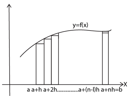
The point of division on $\text{x-}$axis are

$\text{a,a}+\text{h,a}+\text{2h}.....\text{a}+\left( \text{n}-\text{1} \right)\text{h,a}+\text{nh,}$ where $\dfrac{\text{b}-\text{a}}{\text{n}}=\text{h}$.

Let ${{\text{S}}_{\text{n}}}$ denotes the area of these $\text{n}$ rectangles.

Then, ${{\text{S}}_{\text{n}}}=\text{hf(a)}+\text{hf}\left( \text{a}+\text{h} \right)+\text{hf}\left( \text{a}+\text{2h} \right)+....+\text{hf}\left( \text{a}+\left( \text{n}-\text{1} \right)\text{h} \right)$ 

Clearly, ${{\text{S}}_{\text{n}}}$ is area very close to the area of the region bounded by

Curve $\text{y}=\text{f(x),}$ $\text{x-}$axis and the ordinates $\text{x}=\text{a}$, $\text{x}=\text{b}$.

Hence \[\int\limits_{\text{a}}^{\text{b}}{\text{f(x)dx}=\underset{\text{n}\to \infty }{\mathop{\text{Lt}}}\,}{{\text{S}}_{\text{n}}}\] 

\[\int\limits_{\text{a}}^{\text{b}}{\text{f(x)dx}=\underset{\text{n}\to \infty }{\mathop{\text{Lt}}}\,}\sum\limits_{\text{r}=\text{0}}^{\text{n-1}}{\text{hf(a+rh)}}\] 

\[=\underset{\text{n}\to \infty }{\mathop{\text{Lt}}}\,\sum\limits_{\text{r}=\text{0}}^{\text{n-1}}{\left( \dfrac{\text{b}-\text{a}}{\text{n}} \right)}\text{f}\left( \text{a}+\dfrac{\left( \text{b}-\text{a} \right)\text{r}}{\text{n}} \right)\] 

Note:

(a) We can also write

${{\text{S}}_{\text{n}}}=\text{hf}\left( \text{a}+\text{h} \right)+\text{hf}\left( \text{a}+\text{2h} \right)+.....+\text{hf}\left( \text{a}+\text{nh} \right)$ 

\[\int\limits_{\text{a}}^{\text{b}}{\text{f(x)dx}}=\underset{\text{n}\to \infty }{\mathop{\text{Lt}}}\,\sum\limits_{\text{r}=1}^{\text{n}}{\left( \dfrac{\text{b}-\text{a}}{\text{n}} \right)}\text{f}\left( \text{a}+\left( \dfrac{\text{b}-\text{a}}{\text{n}} \right)\text{r} \right)\] 

(b) If \[\text{a}=0,\,\text{b}=1,\,\int\limits_{0}^{1}{\text{f(x)dx}}=\underset{\text{n}\to \infty }{\mathop{\text{Lt}}}\,\sum\limits_{\text{r}=0}^{\text{n}-1}{\dfrac{1}{\text{n}}\text{f}\left( \dfrac{\text{r}}{\text{n}} \right)}\] 

Steps to Express the Limit of Sum as Definite Integral

Step 1. Replace  \[\dfrac{\text{r}}{\text{n}}\] by $\text{x}$, $\dfrac{\text{1}}{\text{n}}$ by $\text{dx}$ and $\underset{\text{n}\to \infty }{\mathop{\text{Lt}}}\,\sum{\text{by}\,}\int{{}}$  

Step 2. Evaluate $\underset{\text{n}\to \infty }{\mathop{\text{Lt}}}\,\left( \dfrac{\text{r}}{\text{n}} \right)$ by putting least and greatest values of $\text{r}$ as lower and upper limits respectively.

For example $\underset{\text{n}\to \infty }{\mathop{\text{Lt}}}\,\sum\limits_{\text{r}=1}^{\text{pn}}{\dfrac{1}{\text{n}}\text{f}\left( \dfrac{\text{r}}{\text{n}} \right)}=\int\limits_{0}{\text{f(x)dx}}$ 

$\left[ \underset{\text{n}\to \infty }{\mathop{\text{Lt}}}\,\left( \dfrac{\text{r}}{\text{n}} \right)\left| _{\text{r}=1}=0,\,\underset{\text{n}\to \infty }{\mathop{\text{Lt}}}\, \right.\left( \dfrac{\text{r}}{\text{n}} \right)\left| _{\text{r}=\text{np}}=\text{p} \right. \right]$ 

5. Reduction Formulae in Definite Integrals

l. If ${{\text{I}}_{\text{n}}}\text{=}\int\limits_{\text{0}}^{\dfrac{\text{ }\!\!\pi\!\!\text{ }}{\text{2}}}{\text{si}{{\text{n}}^{\text{n}}}\text{xdx}}$, then show that ${{\text{I}}_{\text{n}}}\text{=}\left( \dfrac{\text{n}-\text{1}}{\text{n}} \right){{\text{I}}_{\text{n}-\text{2}}}$ 

Proof: ${{\text{I}}_{\text{n}}}\text{=}\int\limits_{\text{0}}^{\dfrac{\text{ }\!\!\pi\!\!\text{ }}{\text{2}}}{\text{si}{{\text{n}}^{\text{n}}}\text{xdx}}$ 

${{\text{I}}_{\text{n}}}\text{=}\left[ -\text{si}{{\text{n}}^{\text{n}-\text{1}}}\text{xcosx} \right]_{\text{0}}^{\dfrac{\text{ }\!\!\pi\!\!\text{ }}{\text{2}}}\text{+}\int\limits_{\text{0}}^{\dfrac{\text{ }\!\!\pi\!\!\text{ }}{\text{2}}}{\left( \text{n}-\text{1} \right)\text{si}{{\text{n}}^{\text{n}-\text{2}}}\text{x}\text{.co}{{\text{s}}^{\text{2}}}\text{xdx}}$ 

$\text{=}\left( \text{n}-\text{1} \right)\int\limits_{\text{0}}^{\dfrac{\text{ }\!\!\pi\!\!\text{ }}{\text{2}}}{\text{si}{{\text{n}}^{\text{n}-\text{2}}}\text{x}\text{.}\left( \text{1}-\text{si}{{\text{n}}^{\text{2}}}\text{x} \right)\text{dx}}$ 

$\text{=}\left( \text{n}-\text{1} \right)\int\limits_{\text{0}}^{\dfrac{\text{ }\!\!\pi\!\!\text{ }}{\text{2}}}{\text{si}{{\text{n}}^{\text{n}-\text{2}}}\text{xdx}-\left( \text{n}-1 \right)\int\limits_{\text{0}}^{\dfrac{\text{ }\!\!\pi\!\!\text{ }}{\text{2}}}{\text{si}{{\text{n}}^{\text{n}}}\text{x}}\text{dx}}$ 

${{\text{I}}_{\text{n}}}+\left( \text{n}-\text{1} \right){{\text{I}}_{\text{n}}}=\left( \text{n}-\text{1} \right){{\text{I}}_{\text{n}-\text{2}}}$ 

${{\text{I}}_{\text{n}}}=\left( \dfrac{\text{n}-\text{1}}{\text{n}} \right){{\text{I}}_{\text{n}-\text{2}}}$ 

Note:

(a) $\int\limits_{\text{0}}^{\dfrac{\text{ }\!\!\pi\!\!\text{ }}{\text{2}}}{\text{si}{{\text{n}}^{\text{n}}}\text{xdx}=\int\limits_{\text{0}}^{\dfrac{\text{ }\!\!\pi\!\!\text{ }}{\text{2}}}{\text{co}{{\text{s}}^{\text{n}}}\text{xdx}}}$ 

(b) ${{\text{I}}_{\text{n}}}=\left( \dfrac{\text{n}-\text{1}}{\text{n}} \right)\left( \dfrac{\text{n}-\text{3}}{\text{n}-\text{2}} \right)\left( \dfrac{\text{n}-\text{5}}{\text{n}-\text{4}} \right)....{{\text{I}}_{\text{0}}}\,\text{or}\,{{\text{I}}_{\text{1}}}$ according as \[\text{n}\] is even or odd, ${{\text{I}}_{\text{0}}}=\dfrac{\text{ }\!\!\pi\!\!\text{ }}{\text{2}}\text{,}\,{{\text{I}}_{\text{1}}}=\text{1}$ 

Hence ${{\text{I}}_{\text{n}}}=\left\{ \begin{matrix} \left( \dfrac{\text{n}-\text{1}}{\text{n}} \right)\left( \dfrac{\text{n}-\text{3}}{\text{n}-\text{2}} \right)\left( \dfrac{\text{n}-\text{5}}{\text{n}-\text{4}} \right).....\left( \dfrac{\text{1}}{\text{2}} \right)\text{.}\dfrac{\text{ }\!\!\pi\!\!\text{ }}{\text{2}}\,\,\text{if}\,\,\text{n}\,\,\text{is}\,\,\text{even}  \\ \left( \dfrac{\text{n}-\text{1}}{\text{n}} \right)\left( \dfrac{\text{n}-\text{3}}{\text{n}-\text{2}} \right)\left( \dfrac{\text{n}-\text{5}}{\text{n}-\text{4}} \right).....\left( \dfrac{\text{2}}{\text{3}} \right)\text{.1}\,\,\text{if}\,\,\text{n}\,\,\text{is }\,\text{odd}  \\ \end{matrix} \right\}$ 

ll. If ${{\text{I}}_{\text{n}}}=\int\limits_{\text{0}}^{\dfrac{\text{ }\!\!\pi\!\!\text{ }}{\text{4}}}{\text{ta}{{\text{n}}^{\text{n}}}\text{xdx}}$, then show that ${{\text{I}}_{\text{n}}}+{{\text{I}}_{\text{n}-\text{2}}}=\dfrac{\text{1}}{\text{n}-\text{1}}$ 

Proof: ${{\text{I}}_{\text{n}}}=\int\limits_{\text{0}}^{\dfrac{\text{ }\!\!\pi\!\!\text{ }}{\text{4}}}{{{\left( \text{tanx} \right)}^{\text{n}-\text{2}}}\text{.ta}{{\text{n}}^{\text{2}}}\text{xdx}}$ 

$=\int\limits_{\text{0}}^{\dfrac{\text{ }\!\!\pi\!\!\text{ }}{\text{4}}}{{{\left( \text{tanx} \right)}^{\text{n}-\text{2}}}\left( \text{se}{{\text{c}}^{\text{2}}}\text{x}-\text{1} \right)\text{dx}}$ 

$\text{=}\int\limits_{\text{0}}^{\dfrac{\text{ }\!\!\pi\!\!\text{ }}{\text{4}}}{{{\left( \text{tanx} \right)}^{\text{n}-\text{2}}}\text{se}{{\text{c}}^{\text{2}}}\text{xdx}}-\int\limits_{\text{0}}^{\dfrac{\text{ }\!\!\pi\!\!\text{ }}{\text{4}}}{{{\left( \text{tanx} \right)}^{\text{n}-\text{2}}}\text{dx}}$ 

$=\left[ \dfrac{{{\left( \text{tanx} \right)}^{\text{n}-\text{1}}}}{\text{n}-\text{1}} \right]_{\text{0}}^{\dfrac{\text{ }\!\!\pi\!\!\text{ }}{\text{4}}}-{{\text{I}}_{\text{n}-\text{2}}}$ 

${{\text{I}}_{\text{n}}}=\dfrac{\text{1}}{\text{n}-\text{1}}-{{\text{I}}_{\text{n}-\text{2}}}$ 

${{\text{I}}_{\text{n}}}+{{\text{I}}_{\text{n}-\text{2}}}=\dfrac{\text{1}}{\text{n}-\text{1}}$ 

lll. If ${{\text{I}}_{\text{m,n}}}=\int\limits_{\text{0}}^{\dfrac{\text{ }\!\!\pi\!\!\text{ }}{\text{2}}}{\text{si}{{\text{n}}^{\text{m}}}\text{x}\text{.co}{{\text{s}}^{\text{n}}}\text{xdx}}$, then show that ${{\text{I}}_{\text{m,n}}}=\dfrac{\text{m}-\text{1}}{\text{m}+\text{n}}{{\text{I}}_{\text{m}-\text{2}}}\text{,n}$ 

Proof: ${{\text{I}}_{\text{m,n}}}=\int\limits_{\text{0}}^{\dfrac{\text{ }\!\!\pi\!\!\text{ }}{\text{2}}}{\text{si}{{\text{n}}^{\text{m}-1}}\text{x}\left( \text{sinxco}{{\text{s}}^{\text{n}}}\text{x} \right)\text{dx}}$ 

$=\left[ -\dfrac{\text{si}{{\text{n}}^{\text{m}-\text{1}}}\text{x}\text{.co}{{\text{s}}^{\text{n}+\text{1}}}\text{x}}{\text{n}+\text{1}} \right]_{\text{0}}^{\dfrac{\text{ }\!\!\pi\!\!\text{ }}{\text{2}}}+\int\limits_{\text{0}}^{\dfrac{\text{ }\!\!\pi\!\!\text{ }}{\text{2}}}{\dfrac{\text{co}{{\text{s}}^{\text{n}+\text{1}}}}{\text{n}+\text{1}}\left( \text{m}-\text{1} \right)\text{si}{{\text{n}}^{\text{m}-\text{2}}}\text{xcosxdx}}$ 

$=\left( \dfrac{\text{m}-\text{1}}{\text{n}+\text{1}} \right)\int\limits_{\text{0}}^{\dfrac{\text{ }\!\!\pi\!\!\text{ }}{\text{2}}}{\text{si}{{\text{n}}^{\text{m}-\text{2}}}\text{x}\text{.co}{{\text{s}}^{\text{n}}}\text{x}\text{.co}{{\text{s}}^{\text{2}}}\text{xdx}}$ 

$=\left( \dfrac{\text{m}-\text{1}}{\text{n}+\text{1}} \right)\int\limits_{\text{0}}^{\dfrac{\text{ }\!\!\pi\!\!\text{ }}{\text{2}}}{\left( \text{si}{{\text{n}}^{\text{m}-\text{2}}}\text{x}\text{.co}{{\text{s}}^{\text{n}}}\text{x}-\text{si}{{\text{n}}^{\text{m}}}\text{x}\text{.co}{{\text{s}}^{\text{n}}}\text{x} \right)\text{dx}}$ 

$=\left( \dfrac{\text{m}-\text{1}}{\text{n}+\text{1}} \right){{\text{I}}_{\text{m}-\text{2,n}}}-\left( \dfrac{\text{m}-\text{1}}{\text{n}+\text{1}} \right){{\text{I}}_{\text{m,n}}}$ 

$\Rightarrow \left( \text{1}+\dfrac{\text{m}-\text{1}}{\text{n}+\text{1}} \right){{\text{I}}_{\text{m,n}}}=\left( \dfrac{\text{m}-\text{1}}{\text{n}+\text{1}} \right){{\text{I}}_{\text{m}-\text{2,n}}}$ 

${{\text{I}}_{\text{m,n}}}\text{=}\left( \dfrac{\text{m}-\text{1}}{\text{m}+\text{n}} \right){{\text{I}}_{\text{m}-\text{2,n}}}$ 

Note:

(a) ${{\text{I}}_{\text{m,n}}}=\left( \dfrac{\text{m}-\text{1}}{\text{m}+\text{n}} \right)\left( \dfrac{\text{m}-\text{3}}{\text{m}+\text{n}-\text{2}} \right)\left( \dfrac{\text{m}-\text{5}}{\text{m}+\text{n}-\text{4}} \right).....{{\text{I}}_{\text{0,n}}}\,\text{or}\,{{\text{I}}_{\text{1,n}}}$ according as $\text{m}$ is even or odd.

${{\text{I}}_{\text{0,n}}}=\int\limits_{\text{0}}^{\dfrac{\text{ }\!\!\pi\!\!\text{ }}{\text{2}}}{\text{co}{{\text{s}}^{\text{n}}}\text{xdx}\,\text{and}\,{{\text{I}}_{\text{1,n}}}=\int\limits_{\text{0}}^{\dfrac{\text{ }\!\!\pi\!\!\text{ }}{\text{2}}}{\text{sinx}\text{.co}{{\text{s}}^{\text{n}}}\text{xdx}=\dfrac{\text{1}}{\text{n+1}}}}$ 

(b) Walli’s Formula

\[{{\text{I}}_{\text{m,n}}}=\left\{ \begin{matrix} \dfrac{\left( \text{m}-\text{1} \right)\left( \text{m}-\text{3} \right)\left( \text{m}-\text{5} \right)....\left( \text{n}-\text{1} \right)\left( \text{n}-\text{3} \right)\left( \text{n}-\text{5} \right)....}{\left( \text{m}+\text{n} \right)\left( \text{m}+\text{n}-\text{2} \right)\left( \text{m}+\text{n}-\text{4} \right).....}\,\,\,\text{when}\,\,\text{both}\,\,\text{m,n}\,\,\text{are}\,\,\text{even}  \\ \dfrac{\left( \text{m}-\text{1} \right)\left( \text{m}-\text{3} \right)\left( \text{m}-\text{5} \right)....\left( \text{n}-\text{1} \right)\left( \text{n}-\text{3} \right)\left( \text{n}-\text{5} \right).....}{\left( \text{m}+\text{n} \right)\left( \text{m}+\text{n}-\text{2} \right)\left( \text{m}+\text{n}-\text{4} \right)....}\,\,\text{otherwise}  \\ \end{matrix} \right\}\] 

Area Under the Curves

(a) Area of Plane Regions:

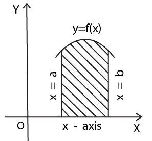
l. The area bounded by the curve $\text{y}=\text{f(x)}$, $\text{x-}$axis and the ordinates $\text{x}=\text{a}$ and \[\text{x}=\text{b}\] (where $\text{ba}$) is given by

$\text{A}=\int\limits_{\text{a}}^{\text{b}}{\left| \text{y} \right|\text{dx}=\int\limits_{\text{a}}^{\text{b}}{\left| \text{f(x)} \right|\text{dx}}}$ 

(i) If $\text{f(x)}>0\forall \text{x}\in \left[ \text{a,b} \right]$ 

Then $\text{A}=\int\limits_{\text{a}}^{\text{b}}{\text{f(x)dx}}$ 

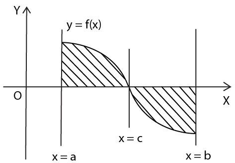
(ii) If $\text{f(x)}>0\forall x\in \left[ \text{a,c} \right)\,\text{ }\!\!\And\!\!\text{ }\,<0\forall \text{x}\in \left( \text{c,b} \right]$ 

Then $\text{A}=\left| \int\limits_{\text{a}}^{\text{c}}{\text{ydx}} \right|+\left| \int\limits_{\text{c}}^{\text{b}}{\text{ydx}} \right|=\int\limits_{\text{a}}^{\text{c}}{\text{f(x)dx}-\int\limits_{\text{c}}^{\text{b}}{\text{f(x)dx}}}$ where $\text{c}$ is a point in between $\text{a}$ and $\text{b}$.

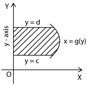
ll. The area bounded by the curve $\text{x}=\text{g(y)}$, $\text{y-}$axis and the abscissae $\text{y}=\text{c}$ and $\text{y}=\text{d}$ (where $\text{dc}$) is given by

$\text{A}=\int\limits_{\text{c}}^{\text{d}}{\left| \text{x} \right|\text{dy}=\int\limits_{\text{c}}^{\text{d}}{\left| \text{g(y)} \right|\text{dy}}}$ 

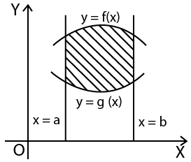
III. If we have two curve $\text{y}=\text{f(x)}$ and $\text{y}=\text{g(x)}$, such that $\text{y}=\text{f(x)}$ lies above the curve $\text{y}=\text{g(x)}$ then the area bounded between them and the ordinates $\text{x}=\text{a}$ and $\text{x}=\text{b}$ $\left( \text{b}>\text{a} \right)$, is given by

$\text{A}=\int\limits_{\text{a}}^{\text{b}}{\text{f(x)dx}-\int\limits_{\text{a}}^{\text{b}}{\text{g(x)dx}}}$ 

i.e. $\text{upper}\,\text{curve}\,\text{area}-\text{lower}\,\text{curve}\,\text{area}$.

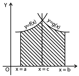
lV. The area bounded by the curves $\text{y}=\text{f(x)}$ and $\text{y}=\text{g(x)}$ between the ordinates $\text{x}=\text{a}$ and $\text{x}=\text{b}$ is given by

$\text{A}=\int\limits_{\text{a}}^{\text{c}}{\text{f(x)dx}+\int\limits_{\text{c}}^{\text{b}}{\text{g(x)dx}}}$, where $\text{x}=\text{c}$ is the point of intersection of the two curves.

V. Curve Tracing

It is necessary to have a rough sketch of the desired piece in order to locate the area enclosed by many curves. The following steps are very useful in tracing a cartesian curve $\text{f(x,y)}=\text{0}$.

Step 1: Symmetry

(i) If all the powers of $\text{y}$ in the equation of the given curve are even then the curve is symmetrical about $\text{x-}$axis.

(ii) If all the powers of $\text{x}$ in the equation of the given curve are even then the curve is symmetrical about $\text{y-}$axis.

(iii) If the equation of the given curve remains unchanged on interchanging $\text{x}$ and $\text{y}$, then the curve is symmetrical about the line\[\text{y}=\text{x}\].

(iv) If the equation of the given curve remains unchanged when $\text{x}$  and $\text{y}$ are replaced by $-\text{x}$  and $-\text{y}$ respectively, then the curve is symmetrical in opposite quadrants.

Step 2: Origin

If the algebraic curve's equation contains no constant term, the curve passes through the origin.

The tangents at the origin are then calculated by equating the lowest degree terms in the equation of the specified algebraic curve to zero.

For example, the curve ${{\text{y}}^{\text{3}}}={{\text{x}}^{\text{3}}}+\text{axy}$ passes through the origin and the tangents at the origin are given by $\text{axy}=0$ i.e. $\text{x}=\text{0}$ and $\text{y}=0$.

Step 3: Intersection with the Co-ordinates Axes

(i) Find out the corresponding values of $\text{x}$ by putting \[\text{y}=\text{0}\] in the equation of the given curve, to estimate the points of intersection of the curve with $\text{x-}$axis

(ii) Find out the corresponding values of $\text{y}$ by putting \[\text{x}=\text{0}\] in the equation of the given curve, to estimate the points of intersection of the curve with $\text{y-}$axis

Step 4: Asymptotes

Find out the asymptotes of the curve.

(i) The vertical asymptotes of the given algebraic curve, or asymptotes parallel to the $\text{y-}$axis, are derived by equating the coefficient of the highest power of $\text{y}$ in the equation of the supplied curve to zero.

(ii) The horizontal asymptotes of the given algebraic curve, or asymptotes parallel to the $\text{x-}$axis, are derived by equating the coefficient of the highest power of $\text{x}$ in the equation of the supplied curve to zero.

Step 5: Region

Find out the regions of the plane in which no part of the curve lies. To determine such regions we solve the given equation for $\text{y}$ in terms of $\text{x}$ or vice-versa. Suppose that y becomes imaginary for\[\text{x}>\text{a}\], the curve does not lie in the region\[\text{x}>\text{a}\].

Step 6: Critical Points

Find out the values of $\text{x}$ at which $\dfrac{\text{dy}}{\text{dx}}=0$ 

At such points $\text{y}$ generally changes its character from an increasing function of $\text{x}$to a decreasing function of $\text{x}$ or vice-versa.

Step 7: 

Trace the curve with the help of the above points.

Important Formulas of Class 12 Chapter 8 You Shouldn’t Miss! 

1. Area Under a Curve:

To find the area between the curve $y = f(x)$ and the x-axis from $x = a$ to $x = b$:

\[\text{Area} = \int_{a}^{b} f(x) \, dx\]

2. Area Between Two Curves:

To find the area between two curves $y = f(x)$ and $y = g(x)$ from $x = a$ to $x = b$:

\[\text{Area}=\mathop{\int }_{a}^{b}[f(x)-g(x)]\,dx\]

3. Volume of a Solid of Revolution:

a. When rotating a curve $y = f(x)$ around the x-axis from $x = a$ to $x = b$:

\[\text{Volume}=\pi \mathop{\int }_{a}^{b}{{[f(x)]}^{2}}\,dx\]

b. When rotating a curve $x = g(y)$ around the y-axis from $y = c$ to $y = d$:

\[\text{Volume}=\pi \mathop{\int }_{c}^{d}{{[g(y)]}^{2}}\,dy\]

4. Length of a Curve:

a. For a curve given by $y = f(x)$ from $x = a$ to $x = b$:

\[\text{Length} = \int_{a}^{b} \sqrt{1 + \left(\frac{dy}{dx}\right)^2} \, dx\]

b. For a curve given by $x = g(y)$ from $y = c$ to $y = d$:

\[\text{Length} = \int_{c}^{d} \sqrt{1 + \left(\frac{dx}{dy}\right)^2} \, dy\]

5. Surface Area of a Solid of Revolution:

a. When rotating a curve y = f(x) around the x-axis from x = a to x = b:

\[\text{Surface }\!\!~\!\!\text{ Area}=2\pi \mathop{\int }_{a}^{b}f(x)\sqrt{1+{{\left( \frac{dy}{dx} \right)}^{2}}}dx\]

b. When rotating a curve x=g(y)x = g(y)x=g(y) around the y-axis from y = c to y = d:

\[\text{Surface }\!\!~\!\!\text{ Area}=2\pi \mathop{\int }_{c}^{d}g(y)\sqrt{1+{{\left( \frac{dx}{dy} \right)}^{2}}}dy\]

Importance of Application of Integrals Class 12 Notes

1. Exam Preparation: The notes highlight important formulas, properties, and problem-solving techniques that are frequently tested in board exams, ensuring students are well-prepared and confident.

2. Foundation for Advanced Topics: The principles learned in this chapter lay the groundwork for more advanced calculus topics and applications in higher studies, including engineering and physics.

3. Quick Revision: The notes provide a concise summary of key concepts, making them an ideal tool for quick revision before exams. This helps in reinforcing learning and recalling important points during the exam.

4. Problem-Solving Skills: By working through examples and exercises included in the notes, students can enhance their analytical and problem-solving skills, which are crucial for tackling complex questions in exams.

5. Conceptual Understanding: Detailed notes provide clear explanations and practical examples, aiding in a deeper understanding of how integrals are applied, which helps in grasping the nuances of the subject.

Tips for Learning the Class 12 Maths Chapter 8 Application of Integrals

Understand the Concepts:

• Begin by thoroughly understanding the basic concepts of integrals. Familiarize yourself with how integrals are used to calculate areas, volumes, and lengths.

Study Key Formulas:

• Memorise and understand the key formulas for calculating areas under curves, volumes of solids of revolution, and lengths of curves. Knowing these formulas will be crucial for solving problems.

Practice Problem-Solving:

• Work on a variety of problems to apply the concepts. Solve exercises that involve different methods, such as the disk method and shell method, to build proficiency.

Visualise Graphs:

• Use graphs to visualize problems involving areas between curves and volumes of revolution. This will help in understanding the application of integrals in a geometric context.

Use Step-by-Step Solutions:

• Study solved examples and work through the steps to understand how problems are approached and solved. Pay attention to the methods and reasoning used.

Conclusion

Mastering the formulas for Class 12 Chapter 8: Application of Integrals is vital for solving complex problems related to areas, volumes, and curve lengths. These formulas provide the foundation for applying integrals to real-world scenarios, helping you excel in exams and develop a deeper understanding of calculus. By thoroughly studying and practising these formulas, you will enhance your problem-solving skills and be well-prepared for both theoretical and practical applications of integrals. Ensure you are familiar with each formula and its application for your exams in this important chapter.

Related Study Materials for Class 12 Maths Chapter 8

Students can also download additional study materials provided by Vedantu for Class 12 Maths Chapter 8 Application of Integrals:

Chapter-wise Revision Notes Links for Class 12 Maths

Important Study Materials for Class 12 Maths