


Physics Notes for Chapter 1 Electric Charges and Fields Class 12 - FREE PDF Download


1. Electric Charge
1.1 Definition- Charge is that property that is associated with the matter due to which it produces and experiences electrical and magnetic effects.
1.2 Type
There exist two types of charges in nature. They are:
i. Positive charge
ii. Negative charge
Charges with the same electrical sign repel each other while charges with opposite electrical signs attract each other.
1.3 Unit and Dimensional Formula
S.I. unit of charge is coulomb (C),
$\left( {1{\text{mC}} = {{10}^{ - 3}}{\text{C}},1\mu {\text{C}} = {{10}^{ - 6}}{\text{C}},\ln {\text{C}} = {{10}^{ - 9}}{\text{C}}} \right)$
C.G.S. the unit of charge is e.s.u. $1{\text{C}} = 3 \times {10^9}$ esu
The Dimensional formula is given by $[{\text{Q}}] = [{\text{AT}}]$.
1.4 Point Charge
Whose spatial size is negligible as compared to other distances.
1.5 Properties of Charge
(i) Charge is a Scalar Quantity: Charges can be added or subtracted algebraically.
(ii) Charge is transferable: When a charged body is put in contact with an uncharged body, the uncharged body becomes charged due to transfer of electrons from the charged body to the uncharged body.
(iii) Charge is always associated with mass: Charge cannot exist without mass though mass can exist without charge.
(iv) Charge is conserved: Charge can neither be created nor be destroyed.
(v) Invariance of charge: The numerical value of an elementary charge is independent of velocity.
(vi) Charge produces an electric field and magnetic field: When a charged particle is at rest it only produces an electric field in the space surrounding it. However, if the charged particle is in unaccelerated motion it produces both electric and magnetic fields. And if the motion of the charged particle is accelerated it not only produces electric and magnetic fields but also radiates energy in the space surrounding the charge in the form of electromagnetic waves.
(vii) Charge resides on the surface of conductor: Charge resides on the outer surface of a conductor because like charges repel and try to get as far away as possible from one another and stay at the farthest distance from each other which is the outer surface of the conductor. Therefore a solid and hollow conducting sphere of the same outer radius will hold a maximum equal charge and a soap bubble expands on charging.
(viii) Quantization of charge: When a physical quantity can have only discrete values rather than any value, the quantity is said to be quantised. The smallest charge that can exist in nature is the charge of an electron. If the charge of an electron $\left( { - 1.6 \times {{10}^{ - 19}}{\text{C}}} \right)$ is taken as elementary unit i.e. quanta of charge the charge on anybody will be some integral multiple of e i.e., ${\text{Q}} = \pm ne$ with ${\text{n}} = 0$, $1,2,3 \ldots \ldots $
Charge on a body can never be $0.5\,e,\, \pm 17.2e$ or $ \pm {10^{ - 5}}e$ etc.
1.6 Comparison of Charge and Mass
We are familiar with the role of mass in gravitation and we have just studied some features of electric charge. The comparison between the two are as follows:
1.7 Methods of Charging
A body can be charged by following methods:
i. By friction:
In friction when two bodies are rubbed together, electrons are transferred from one body to the other. As a result of this one body becomes positively charged while the other is negatively charged, e.g., when a glass rod is rubbed with silk, the rod becomes positively charged while the silk becomes negatively charged. However, ebonite on rubbing with wool becomes negatively charged making the wool positively charged. Clouds also become charged by friction. In charging by friction in accordance with conservation of charge, both positive and negative charges in equal amounts appear simultaneously due to the transfer of electrons from one body to the other.
ii. By electrostatic induction:
If a charged body is brought near an uncharged body, the charged body will attract the opposite charge and repel a similar charge present in the uncharged body. As a result of this one side of the neutral body (closer to charged body) becomes oppositely charged while the other is similarly charged. This process is called electrostatic induction.
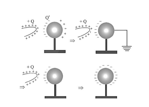
Note: Inducting body neither gains nor loses charge.
(iii) Charging by conduction:
Take two conductors, one charged and the other uncharged. Bring the conductors in contact with each other. The charge (whether negative or positive) under its own repulsion will spread over both the conductors. Thus, the conductors will be charged with the same sign. This is called as charging by conduction (through contact).
Note: A truck carrying explosives has a metal chain touching the ground, to conduct away the charge produced by friction.
2. Coulomb's Law
If two stationary and point charges ${Q_1}$ and ${Q_2}$ are kept at a distance $r$, then it is found that force of attraction or repulsion between them is Mathematically, Coulomb's law can be written as
${\text{F}} = {\text{k}}\dfrac{{{{\text{q}}_1}{{\text{q}}_2}}}{{{{\text{r}}^2}}}$
where ${\text{k}}$ is a proportionality constant.
In SI units ${\text{k}}$ has the value,
${\text{k}} = 8.988 \times {10^9}{\text{N}}{{\text{m}}^2}/{{\text{C}}^2}$
${\text{k}} = 9.0 \times {10^9}{\text{N}}{{\text{m}}^2}/{{\text{C}}^2}$
(a) The direction of force is always along the line joining the two charges.
(b) The force is repulsive if the charges have the same sign and attractive if their signs are opposite.
(c) This force is conservative in nature.
(d) This is also called inverse square law.
2.1 Variation of $k$
Constant $k$ depends upon a system of units and medium between the two charges.
In C.GS. for air
$k=1,\;{\text{F}}=\dfrac{{{{\text{Q}}_1}{{\text{Q}}_2}}} {{{{\text{r}}^2}}} {\text{Dyne}}$
In S.I. for air $k = \dfrac{1}{{4\pi {\varepsilon _0}}} = 9 \times {10^9}\dfrac{{{\text{N}} - {{\text{m}}^2}}}{{{{\text{C}}^2}}}$,
${\text{F}} = \dfrac{1}{{4\pi {\varepsilon _0}}} \cdot \dfrac{{{{\text{Q}}_1}{{\text{Q}}_2}}}{{{{\text{r}}^2}}}{\text{ Newton }}\left( {1{\text{ Newton }} = {{10}^5}} \right.{\text{ Dyne) }}$
Note:
${\varepsilon _0} = $ Absolute permittivity of air or free space
$ = 8.85 \times {10^{ - 12}}\dfrac{{{C^2}}}{{N - {m^2}}}\left( { = \dfrac{{{\text{ Farad }}}}{m}} \right)$
Dimension is $\left[ {{M^{ - 1}}{L^{ - 3}}{T^4}{A^2}} \right]$
${\varepsilon _0}$ Relates with absolute magnetic permeability $\left( {{\mu _0}} \right)$ and velocity of light $(c)$ according to the following relation $c = \dfrac{1}{{\sqrt {{\mu _0}{\varepsilon _0}} }}$
2.1.2 Effect of Medium
(a) When a dielectric medium is completely filled in between charges rearrangement of the charges inside the dielectric medium takes place and the force between the same two charges decreases by a factor of $K$ known as dielectric constant, $K$ is also called relative permittivity ${\varepsilon _r}$ of the medium (relative means with respect to free space).
Hence in the presence of medium
${F_m} = \dfrac{{{F_{{\text{air }}}}}}{K} = \dfrac{1}{{4\pi {\varepsilon _0}K}} \cdot \dfrac{{{Q_1}{Q_2}}}{{{r^2}}}$
Here ${\varepsilon _0}\;{\text{K}} = {\varepsilon _0}{\varepsilon _{\text{r}}} = \varepsilon $ (permittivity of medium)
2.2 Vector Form of Coulomb's Law
It is helpful to adopt a convention for subscript notation.
${{\text{F}}_{12}} = $ force on 1 due to $2\quad \;{{\text{F}}_{21}} = $ force on 2 due to 1
(Image will be uploaded soon)
Suppose the position vectors of two charges ${{\text{q}}_1}$ and ${{\text{q}}_2}$ are ${\overrightarrow {\text{r}} _1}$ and ${\overrightarrow {\text{r}} _2}$, then, electric force on charge ${{\text{q}}_1}$ due to charge ${{\text{q}}_2}$ is,
${\overrightarrow {\text{F}} _{12}} = \dfrac{1}{{4\pi {\varepsilon _0}}}\dfrac{{{q_1}{q_2}}}{{{{\left| {{{\overrightarrow {\text{r}} }_1} - {{\overrightarrow {\text{r}} }_2}} \right|}^3}}}\left( {{{\overline {\text{r}} }_1} - {{\overrightarrow {\text{r}} }_2}} \right)$
Similarly, electric force on ${{\text{q}}_2}$ due to charge ${{\text{q}}_1}$ is
${{\text{\vec F}}_{{\text{21}}}} = \dfrac{1}{{4\pi {\varepsilon _0}}}\dfrac{{{q_1}{q_2}}}{{{{\left| {{{\vec r}_2} - {{\vec r}_1}} \right|}^3}}}\left( {{{\vec r}_2} - {{\vec r}_1}} \right)$
Force is a vector, so in vector form the Coulomb's law is written as
${\overrightarrow {\text{F}} _{12}} = \dfrac{1}{{4\pi {\varepsilon _0}}}\dfrac{{{{\text{q}}_1}{{\text{q}}_2}}}{{{{\text{r}}^2}}}{\widehat {\text{r}}_{12}}$
Where ${\widehat {\text{r}}_{12}}$ is a unit vector, directed toward ${{\text{q}}_1}$ from ${{\text{q}}_2}$.
Note:
\[{\widehat r_{12}} = - {\widehat r_{21}}\]
\[{\overrightarrow {\text{F}} _{12}} = \dfrac{1}{{4\pi {\varepsilon _0}}}\dfrac{{{{\text{q}}_1}{{\text{q}}_2}}}{{{{\text{r}}^2}}}{\widehat {\text{r}}_{12}} = \dfrac{1}{{4\pi {\varepsilon _0}}}\dfrac{{{{\text{q}}_2}{{\text{q}}_1}}}{{{{\text{r}}^2}}}\left( { - {{\widehat {\text{r}}}_{21}}} \right)\]
\[{\overrightarrow {\text{F}} _{12}} = - \dfrac{1}{{4\pi {\varepsilon _0}}}\dfrac{{{{\text{q}}_2}{{\text{q}}_1}}}{{{{\text{r}}^2}}}{\widehat {\text{r}}_{21}} = - {\overrightarrow {\text{F}} _{21}} \]
Remember convention for $\widehat {\text{r}}$.
Here ${q_1}$ and ${q_2}$ are to be substituted with sign. Position vector of charges ${q_1}$ and ${q_2}$ are ${\vec r_1} = {x_1}\hat i + {y_1}\hat j + {z_1}\hat k$ and ${\vec r_2} = {x_2}\hat i + {y_2}\hat j + {z_2}\hat k$ respectively. Where $\left( {{x_1},{y_1},{z_1}} \right)$ and $\left( {{x_2},{y_2},\,\,{z_2}} \right)$ are the co-ordinates of charges ${{\text{q}}_1}$ and ${{\text{q}}_2}$.
2.3 Principle of Superposition
According to the principle of superposition, the total force acting on a given charge due to a number of charges is the vector sum of the individual forces acting on that charge due to all the charges.
Consider number of charges Q1, Q2, Q3…..are applying force on a charge $Q$
Net force on $Q$ will be
${\overrightarrow {\text{F}} _{{\text{net }}}} = {\overrightarrow {\text{F}} _1} + {\overrightarrow {\text{F}} _2} + \ldots \ldots \ldots + {\overrightarrow {\text{F}} _{{\text{n}} - 1}} + {\overrightarrow {\text{F}} _{\text{n}}}$
The magnitude of the resultant of two electric force is given by ${\text{F}} = \sqrt {{\text{F}}_1^2 + {\text{F}}_2^2 + 2\;{{\text{F}}_1}\;{{\text{F}}_2}\cos \theta } $ and the force direction is given by,
$\tan \alpha = \dfrac{{{F_2}\sin \theta }}{{{F_1} + {F_2}\cos \theta }}$
3. Electric Field
A positive charge or a negative charge is said to create its field around itself. Thus space around a charge in which another charged particle experiences a force is said to have an electrical field in it.
3.1 Electric Field Intensity $\left( {\overrightarrow {\text{E}} } \right)$
The electric field intensity at any point is defined as the force experienced by a unit positive charge placed at that point.
$\vec E = \dfrac{{\vec F}}{{{q_0}}}$
Where ${q_0} \to 0$ so that presence of this charge may not affect the source charge $Q$ and its electric field is not changed, therefore expression for electric field intensity can be better written as:
$\vec E = \mathop {\lim }\limits_{{q_0} \to 0} \dfrac{{\vec F}}{{{q_0}}}$
(a) Unit and Dimensional formula:
It's S.I. unit is,
$\dfrac{{{\text{ Newton }}}}{{{\text{ coulomb }}}} = \dfrac{{{\text{ volt }}}}{{{\text{ meter }}}} = \dfrac{{{\text{ Joule }}}}{{{\text{ coulomb }} \times {\text{ meter }}}}$ and
C.G.S. unit =${\text{Dyne/stat}}\,\,{\text{coulomb}}.$
Dimension: $\left[ {\text{E}} \right] = \left[ {{\text{ML}}{{\text{T}}^{ - 3}}{{\text{A}}^{ - 1}}} \right]$
(b) Direction of electric field: Electric field (intensity) $\overrightarrow {\text{E}} $ is a vector quantity. Electric field due to a positive charge is always away from the charge and that due to a negative charge is always towards the charge.
3.2 Relation Between Electric Force and Electric Field
In an electric field ${\text{\vec E}}$ a charge $(Q)$ experiences a force $F = QE$. If the charge is positive then force is directed in the direction of the field while if the charge is negative force acts on it in the opposite direction of field.
3.3 Superposition of Electric Field
The resultant electric field at any point is equal to the vector sum of electric fields at that point due to various charges.
$\overrightarrow {\text{E}} = {\overrightarrow {\text{E}} _1} + {\overrightarrow {\text{E}} _2} + {\overrightarrow {\text{E}} _3} + \ldots $
The magnitude of the resultant of two electric fields are given by
${\text{E}} = \sqrt {{\text{E}}_1^2 + {\text{E}}_2^2 + 2{{\text{E}}_1}{{\text{E}}_2}\cos \theta } $ and the direction is given by,
$\tan \alpha = \dfrac{{{E_2}\sin \theta }}{{{E_1} + {E_2}\cos \theta }}$
3.4 Point Charge
Point charge produces its electric field at a point ${\text{P}}$ which is distance $r$ from it given by,
${{\text{E}}_{\text{P}}} = \dfrac{{\text{Q}}}{{4\pi {\varepsilon _0}{{\text{r}}^2}}}$ (Magnitude)
For positive point charge, ${\text{E}}$ is directed away from it.
For negative point charge, ${\text{E}}$ is directed towards it.
3.5 Continuous Charge Distributions
There is an infinite number of ways in which we can spread a continuous charge distribution over a region of space. Mainly three types of charge distributions will be used. We define three different charge densities.
If a total charge $q$ is distributed along a line of length $\ell $, over a surface area A or throughout a volume V, we can calculate charge densities from.
$\lambda = \dfrac{{\text{q}}}{\ell },\sigma = \dfrac{{\text{q}}}{{\text{A}}},\rho = \dfrac{{\text{q}}}{{\text{V}}}$
3.6 Properties of Electric Field Lines
1. Electric field lines originate from a positive charge & terminate on a negative charge.
2. The number of field lines originating/terminating on a charge is proportional to the magnitude of the charge.
3. The number of Field Lines passing through the perpendicular unit area will be proportional to the magnitude of the Electric Field there.
4. Tangent to a Field line at any point gives the direction of the Electric Field at that point. This will be the instantaneous path charge will take if kept there.
5. Two or more field lines can never intersect each other.
(they cannot have multiple directions)
6. Uniform field lines are straight, parallel & uniformly placed.
7. Field lines cannot form a loop.
8. Electric field lines originate and terminate perpendicular to the surface of the conductor. Electric field lines do not exist inside a conductor.
9. Field lines always flow from higher potential to lower potential.
10. If in a region electric field is absent, there will be no field lines.
3.7 Motion of Charged Particle in an Electric Field
(a) When charged particle initially at rest is placed in the uniform field:
Let a charge particle of mass $m$ and charge $Q$ be initially at rest in an electric field of strength $E$.
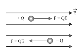
(i) Force and acceleration:
The force experienced by the charged particle is $F = QE$. Positive charge experiences force in the direction of electric field while negative charge experiences force in the direction opposite to the field. [Fig. (A)]
Acceleration produced by this force is ${\text{a}} = \dfrac{{\text{F}}}{{\text{m}}} = \dfrac{{{\text{QE}}}}{{\text{m}}}$
Since the field ${\text{E}}$ in constant the acceleration is constant, thus motion of the particle is uniformly accelerated.
(ii) Velocity:
Suppose at point $A$ particle is at rest and in time $t$, it reaches the point $B$
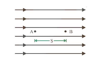
$V = $ Potential difference between $A$ and $B$
$S = $ Separation between $A$ and $B$
(a) By using
$v = {\text{u}} + {\text{at}},\quad v = 0 + {\text{Q}}\dfrac{{\text{E}}}{{\text{m}}}$
${\text{t}} \Rightarrow v = \dfrac{{{\text{QEt}}}}{{\text{m}}}$
(b) By using,
${{\text{v}}^{\text{2}}}{\text{ = }}{{\text{u}}^{\text{2}}}{\text{ + 2as,}}{{\text{v}}^{\text{2}}}{\text{ = 0 + 2 \times }}\dfrac{{{\text{QE}}}}{{\text{m}}}{\text{ \times s = }}\sqrt {\dfrac{{{\text{2QEs}}}}{{\text{m}}}} $
(iii) Momentum:
Momentum $p = mv$,
${\text{p}} = {\text{m}} \times \dfrac{{{\text{QEt}}}}{{\text{m}}} = {\text{QEt}}$
(iv) Kinetic energy:
Kinetic energy gained by the particle in time $t$ is
${\text{K}} = \dfrac{1}{2}{\text{m}}{{\text{v}}^2} = \dfrac{1}{2}\;{\text{m}}\dfrac{{{{({\text{QEt}})}^2}}}{{\;{\text{m}}}} = \dfrac{{{{\text{Q}}^2}{{\text{E}}^2}{{\text{t}}^2}}}{{2\;{\text{m}}}}$
(b) When a charged particle enters with an initial velocity at a right angle to the uniform field.
When a charged particle enters perpendicularly in an electric field, it describes a parabolic path as shown.
(i) Equation of trajectory:
Throughout the motion, a particle has uniform velocity along$x$-axis and horizontal displacement$(x)$ is given by the equation $x = ut$
Since the motion of the particle is accelerated along $y$-axis, we will use the equation of motion for uniform acceleration to determine displacement y.
From ${\text{S}} = {\text{ut}} + \dfrac{1}{2}{\text{a}}{{\text{t}}^2}$
We have $u = 0$ (along $y - $axis) so $y = \dfrac{1}{2}a{t^2}$
i.e., displacement along $y$-axis will increase rapidly with time (since y $\left. { \propto {{\text{t}}^2}} \right)$
From displacement along ${\text{x}}$-axis, ${\text{t}} = {\text{x}}/{\text{u}}$
So $y = \dfrac{1}{2}\left( {\dfrac{{QE}}{m}} \right){\left( {\dfrac{x}{u}} \right)^2};$ this is the equation of parabola which shows ${\text{y}} \propto {{\text{x}}^2}$.
(ii) Velocity at any instant:
At any instant $t,{v_x} = u$ and ${v_{\text{y}}} = \dfrac{{{\text{QEt}}}}{{\text{m}}}$.
So,
$v = |\vec v| = \sqrt {v_{\text{x}}^2 + v_{\text{y}}^2} = \sqrt {{{\text{u}}^2} + \dfrac{{{{\text{Q}}^2}{{\text{E}}^2}{{\text{t}}^2}}}{{\;{{\text{m}}^2}}}} $
If $\beta $ is the angle made by $v$ with $x$-axis than
$\tan \beta = \dfrac{{{v_y}}}{{{v_x}}} = \dfrac{{{\text{QEt}}}}{{{\text{mu}}}}{\text{.}}$
7. Electric Dipole
7.1 General Information
A system of two equal and opposite charges separated by a small fixed distance is called a dipole.
(i) Dipole axis: Line joining negative charge to positive charge of a dipole is called its axis. It may also be termed as its longitudinal axis.
(ii) Equatorial axis: Perpendicular bisector of the dipole is called its equatorial or transverse axis as it is perpendicular to the length.
(iii). Dipole length: The distance between two charges is known as dipole length (d).
(iv). Dipole moment: It is a quantity that gives information about the strength of dipole. It is a vector quantity and is directed from negative charge to positive charge along the axis. It is denoted as p and is defined as the product of the magnitude of either of the charge and the dipole length.
i.e., $\vec p = q(\vec d)$
Its S.I. unit is coulomb-metre or Debye (1 Debye = $\left. {3.3 \times {{10}^{ - 30}}C \times m} \right)$ and its dimensions are ${M^0}{L^1}{T^1}{A^1}$.
Note:
A region surrounding a stationary electric dipole has electric field only.
When a dielectric is placed in an electric field, its atoms or molecules are considered as tiny dipoles.
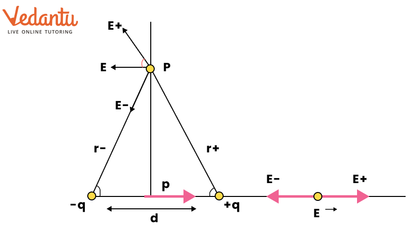
(b) Electric Field due to dipole
(i) For points on the axis
Let the point ${\text{Pbe}}$ at distance ${\text{r}}$ from the centre of the dipole on the side of the charge $q$,as shown in the below figure.
Then
${E_{ - q}} = - \dfrac{q}{{4\pi {z_0}{{(r + a)}^2}}}\hat p$
where $\widehat {\text{p}}$ is the unit vector along the dipole axis (from \[ - q\] to \[q\] ). Also, ${{\text{E}}_{ + {\text{q}}}} = \dfrac{{\text{q}}}{{4\pi {\varepsilon _0}{{({\text{r}} - {\text{a}})}^2}}}\widehat {\text{p}}$
The total field at P is,
\[E = {E_{ + q}} + {E_{ - q}} = \dfrac{q}{{4\pi {\varepsilon _0}}}\left[ {\dfrac{1}{{{{(r - a)}^2}}} - \dfrac{1}{{{{(r + a)}^2}}}} \right]\hat p \]
\[= \dfrac{q}{{4\pi {\varepsilon _0}}}\dfrac{{4ar}}{{{{\left( {{r^2} - {a^2}} \right)}^2}}}\hat p \]
For $r >> a$
$E = \dfrac{{4qa}}{{4\pi {\varepsilon _0}{r^3}}}\hat p\quad (r > > a)$…(i)
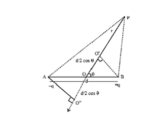
(ii) For points on the equatorial plane
The magnitudes of the electric fields due to the two charges $ + {\text{q}}$ and $ - {\text{q}}$ are given by,
\[{E_{ + q}} = \dfrac{q}{{4\pi {\varepsilon _0}}}\dfrac{1}{{{r^2} + {a^2}}} \]
\[{E_{ - q}} = \dfrac{q}{{4\pi {\varepsilon _0}}}\dfrac{1}{{{r^2} + {a^2}}} \]
and are equal.
The directions of ${E_{ + q}}$ and ${E_{ - q}}$ are as shown in fig. (b). Clearly, the components normal to the dipole axis cancel away. The components along the dipole axis add up. The total electric field is opposite to $\widehat {\text{p}}$. We have,
\[{\text{E}} = - \left( {{{\text{E}}_{ + {\text{q}}}} + {{\text{E}}_{ - \alpha }}} \right)\cos \theta \widehat {\text{p}} \]
\[= - \dfrac{{2{\text{qa}}}}{{4\pi {\varepsilon _0}{{\left( {{{\text{r}}^2} + {{\text{a}}^2}} \right)}^{3/2}}}}\widehat {\text{p}} \]
At large distances $(r > > a)$, this reduces to
$E = - \dfrac{{2qa}}{{4\pi {\varepsilon _0}{r^3}}}{\hat p_{(r > > a)}}$…(ii)
From Eqs. (i) and (ii), it is clear that the dipole field at large distances does not involve $q$ and a separately; it depends on the product $qa$. This suggests the definition of dipole is defined by
${\text{P}} = {\text{q}} \times 2{\text{a}}\widehat {\text{p}}$
that is, it is a vector whose magnitude is charge $q$ times the separation $2a$ (between the pair of charges $q$, $ - q$) and the direction is along the line from $ - q$ to $q$. In tarms of p, the electric field of a dipole at large distances takes simple forms:
At a point on the dipole axis
$E = \dfrac{{2p}}{{4\pi {\varepsilon _0}{r^3}}} = \dfrac{{2kp}}{{{r^3}}}(r > > a)$
At a point on the equatorial plane.
${\text{E}} = \dfrac{{\text{p}}}{{4\pi {\varepsilon _0}{{\text{r}}^3}}} = \dfrac{{ - {\text{kp}}}}{{{{\text{r}}^3}}}({\text{r}} > > {\text{a}})$
7.3 Electric Dipole in a Uniform Electric Field
(i) Force and Torque: If a dipole is placed in a uniform field such that dipole (i.e. $\vec p$ ) makes an angle $\theta $ with the direction of field then two equal and opposite forces acting on dipole constitute a couple whose tendency is to rotate the dipole hence torque is developed in it and dipole tries to align itself in the direction of the field. Consider an electric dipole in placed in a uniform electric field such that dipole (i.e., $\vec p$) makes an angle $\theta $ with the direction of the electric field as shown.
(a) Net force on electric dipole ${{\text{F}}_{{\text{net}}}} = 0$
(b) $\quad \ldots \ldots \quad \tau = {\text{pE}}\sin \theta (\vec \tau = \overrightarrow {\text{p}} \times \overrightarrow {\text{E}} )$
(ii) Work: From the above discussion it is clear that in an uniform electric field dipole tries to align itself in the direction of electric field (i.c. equilibrium position). To change it's angular position some work has to be done.
Suppose an electric dipole is kept in an uniform electric field by making an angle ${\theta _1}$ with the field, if it is again turn so that it makes an angle ${\theta _2}$ with the field, work done in this process is given by the formula
${\text{W = qE}}\left( {{\text{cos}}{{\text{\theta }}_{\text{1}}} - {\text{cos}}{{\text{\theta }}_{\text{2}}}} \right)$
(iii) Potential energy: In case of a dipole (in a uniform field), potential energy of dipole is defined as work done in rotating a dipole from a direction perpendicular to the field to the given direction i.e. if ${\theta _1} = {90^o}$ and ${\theta _2} = \theta $ then
$W=\delta U={U_{\theta}}-{U_{90^o}}=-PE \cos \theta $
$ \Rightarrow {U_{\theta}}= -PE \cos \theta \left ( \because U_{90}=0\:or\:U=-PE \right )$
8.2 Neutral Point
A neutral point is a point where resultant electrical field is zero. Thus neutral points can be obtained only at those points where the resultant field is subtractive.
(a) At an internal point along the line joining two like charges (Due to a system of two like point charge): Suppose two like charges. ${Q_1}$ and ${Q_2}$ are separated by a distance ${\text{x}}$ from each other along a line as shown in following figure.
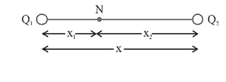
If ${\text{N}}$ is the neutral point at a distance ${{\text{x}}_1}$ from ${{\text{Q}}_1}$ and at a distance ${x_2}\left( { = x - {x_1}} \right)$ from ${Q_2}$ then for natural pt. at $N$,
| E.F. due to ${Q_1}| = |E.F$ due to ${Q_2}\mid $ i.e.,
$\dfrac{1}{{4\pi {\varepsilon _0}}} \cdot \dfrac{{\left| {{Q_1}} \right|}}{{x_1^2}} = \dfrac{1}{{4\pi {\varepsilon _0}}} \cdot \dfrac{{\left| {{Q_2}} \right|}}{{x_2^2}} \Rightarrow \dfrac{{\left| {{Q_1}} \right|}}{{\left| {{Q_2}} \right|}} = {\left( {\dfrac{{{x_1}}}{{{x_2}}}} \right)^2}$
Short trick:
${x_1} = \dfrac{x}{{1 + \sqrt {\left| {{Q_2}} \right|/\left| {{Q_1}} \right|} }}{\text{ and }}{x_2} = \dfrac{x}{{1 + \sqrt {{Q_1}|/|{Q_2}\mid } }}$
Note:
In the above formula if ${Q_1} = {Q_2}$, neutral point lies at the centre so remember that resultant field at the midpoint of two equal and like charges is zero.
(b) At an external point along the line joining two unlike charges (Due to a system of two unlike point charge):
Suppose two unlike charge ${Q_1}$ and ${Q_2}$ separated by a distance $x$ from each other.
Here neutral point lies outside the line joining two unlike charges and also it lies nearer to charge which is smaller in magnitude.
If $\left| {{Q_1}} \right| < \mid {Q_2}$ then neutral point will be obtained on the side of ${Q_1}$, suppose it is at a distance $l$ from ${Q_1}$ Hence at neutral point;
$\dfrac{{{\text{k}}\left| {{Q_1}} \right|}}{{{\ell ^2}}} = \dfrac{{{\text{k}}\left| {{{\text{Q}}_2}} \right|}}{{{{(x + \ell )}^2}}} \Rightarrow \dfrac{{\left| {{Q_1}} \right|}}{{\left| {{Q_2}} \right|}} = {\left( {\dfrac{\varepsilon }{{x + 2}}} \right)^2}$
Short trick: $\ell = \dfrac{x}{{\left( {\sqrt {{Q_2}\left| {/{Q_1}} \right|} - 1} \right)}}$
Note:
In the above discussion if $\left| {{Q_1}} \right| = \left| {{Q_2}} \right|$ neutral point will be at infinity.
8.3 Equilibrium of Charge
(a) Definition: A charge is said to be in equilibrium, if net force acting on it is zero. A systern of charges is said to be in equilibrium if each charge is in equilibrium.
(b) Type of equilibrium: Equilibrium can be divided in following type:
(i) Stable equilibrium: After displacing a charged particle from it's equilibrium position, if it returns back then it is said to be in stable equilibrium. If ${\text{U}}$ is the potential energy then in case of stable equilibrium ${\mathbf{U}}$ is minimum.
(ii) Unstable equilibrium: After displacing a charged particle from it's equilibrium position, if it never returns back then it is said to be in unstable equilibrium and in unstable equilibrium, U is maximum.
(iii) Neutral equilibrium: After displacing a charged particle from it's equilibrium position if it neither comes back, nor moves away but remains in the position in which it was kept it is said to be in neutral equilibrium and in neutral equilibrium, U is constant.
(c) Different cases of equilibrium of charge
Suppose three similar charges ${Q_1},q$ and ${Q_2}$ are placed along a straight line as shown below.
Case -1:
Charge $q$ will be in equilibrium if $\left| {{{\text{F}}_1}} \right| = \left| {{{\text{F}}_2}} \right|$ ie.,,$\dfrac{{{{\text{Q}}_1}}}{{{{\text{Q}}_2}}} = {\left( {\dfrac{{{{\text{x}}_1}}}{{{{\text{x}}_2}}}} \right)^2}$;
This is the condition of equilibrium of charge $q$. After following the guidelines, we can say that charge $q$ is in stable equilibrium and this system is not in equilibrium.
${x_1} = \dfrac{x}{{1 + \sqrt {{Q_2}/{Q_1}} }}{\text{ and }}{x_2} = \dfrac{x}{{1 + \sqrt {{Q_1}/{Q_2}} }}$
e.g. if two charges $ + 4\mu C$ and $ + 16\mu C$ are separated by a distance of $30\;{\text{cm}}$ from each other then for equilibrium a third charge should be placed between them at a distance
${{\text{x}}_1} = \dfrac{{30}}{{1 + \sqrt {16/4} }} = 10\;{\text{cm or }}{{\text{x}}_2} = 20\;{\text{cm}}$
Case-2:
Two similar charge ${{\text{Q}}_1}$ and ${{\text{Q}}_2}$ are placed along a straight line at a distance $x$ from each other and a third dissimilar charge $q$ is placed in between them as shown below
Charge $g$ will be in equilibrium if $\left| {{{\text{F}}_1}} \right| = \left| {{{\text{F}}_2}} \right|$
i.e., $\dfrac{{{Q_1}}}{{{Q_2}}} = {\left( {\dfrac{{{x_1}}}{{{x_2}}}} \right)^2}$.
Note:
Same short trick can be used here to find the position of charge $q$ as we discussed in Case-1 i.e.,
${x_1} = \dfrac{x}{{1 + \sqrt {{Q_2}/{Q_1}} }}$ and ${x_2} = \dfrac{x}{{1 + \sqrt {{Q_1}/{Q_2}} }}$
It is very important to know that magnitude of charge $q$ can be determined if one of the extreme charge (either ${Q_1}$. or $\left. {{Q_2}} \right)$ is in equilibrium ie. if ${Q_2}$ is in equilibrium then$\left| q \right| = {{\text{Q}}_1}{\left( {{{\text{x}}_2}/{\text{x}}} \right)^2}$ and if ${{\text{Q}}_1}$ is in equilibrium then $|{\text{q}}| = {{\text{Q}}_2}{\left( {{{\text{x}}_1}/{\text{x}}} \right)^2}({\text{It}}$ should be remember that sign of $q$ is opposite to that of $\left. {{Q_1}\left( {{\text{or }}{Q_2}} \right)} \right)$.
Case -3:
Two dissimilar charge ${Q_1}$ and ${Q_2}$ are placed along a straight line at a distance ${\text{x}}$ from each other, a third charge q should be placed outside the line joining ${Q_1}$ and ${Q_2}$ for it to experience zero net force.
(Let $\left. {\left| {{Q_2}} \right| < \mid {Q_1}} \right)$
Short Trick :
For it's equilibrium. Charge $q$ lies on the side of charge which is smallest in magnitude and
$d = \dfrac{x}{{\sqrt {{Q_1}/{Q_2} - 1} }}$
11. Electric Dipole
11.1 Electric Field Due to a Dipole
Using the concept that if we know potential electric field can be calculated we have already calculated
${{\text{V}}_{\text{p}}} = \dfrac{{{\text{kp}}\cos \theta }}{{{{\text{r}}^2}}}$
To Calculate net electric field at P we need ${\text{E}}$ (Radial Component) & ${E_1}$ (tangential component) of electric field at P.
${{\text{E}}_{\text{r}}} = \dfrac{{ - {\text{dV}}}}{{{\text{dr}}}}.$ (When we travel in the radial direction).
${{\text{E}}_{\text{t}}} = - \dfrac{{{\text{dV}}}}{{{\text{rd}}\theta }}$ (When we travel in the tangential direction).
\[{{\text{V}}_{\text{p}}} = \dfrac{{{\text{kP}}\cos \theta }}{{{{\text{r}}^2}}} \]
\[ {{\text{E}}_{\text{r}}} = \dfrac{{ - {\text{d}}}}{{{\text{dr}}}}\left( {\dfrac{{{\text{kP}}\cos \theta }}{{{{\text{r}}^2}}}} \right) = \dfrac{{2{\text{kP}}\cos \theta }}{{{{\text{r}}^3}}}\]
${{\text{E}}_{\text{t}}} = \dfrac{{ - {\text{d}}}}{{{\text{rd}}\theta }}\left( {\dfrac{{{\text{kP}}\cos \theta }}{{{{\text{r}}^2}}}} \right) = \dfrac{{ - {\text{kP}}}}{{{{\text{r}}^3}}}\dfrac{{\text{d}}}{{{\text{d}}\theta }}\cos \theta = \dfrac{{{\text{kP}}\sin \theta }}{{{{\text{r}}^3}}}$
${E_{{\text{net }}}} = \sqrt {E_r^2 + E_t^2} = \sqrt {{{\left( {\dfrac{{kP}}{{{r^3}}}} \right)}^2}\left[ {4{{\cos }^2}\theta + {{\sin }^2}\theta } \right]} $
${E_{net}} = \sqrt {{{\left( {\dfrac{{kP}}{{{r^3}}}} \right)}^2}\left[ {1 + 3{{\cos }^2}\theta } \right]} $
${E_{net}} = \dfrac{{kP}}{{{r^3}}}\sqrt {1 + 3{{\cos }^2}\theta } $
(Image will be uploaded soon)
$\tan \alpha = \dfrac{{{E_t}}}{{{E_r}}} = \dfrac{{\dfrac{{kP}}{{{r^3}}}\sin \theta }}{{2\dfrac{{kP\cos \theta }}{{{r^3}}}}} = \dfrac{{\tan \theta }}{2}\quad \alpha = {\tan ^{ - 1}}\left[ {\dfrac{{\tan \theta }}{2}} \right]$
(Note: $\alpha $ is the angle with the radial direction)
11.2 Equilibrium of Dipole
We know that, for any equilibrium net torque and net force on a particle (or system) should be zero.
We already discussed when a dipole is placed in an uniform electric field net force on dipole is always zero. But net torque will be zero only when $\theta = {0^o }$ or ${180^0 }$.
When $\theta = {0^o }$ i.e., dipole is placed along the electric field it is said to be in stable equilibrium, because after turning it through a small angle, dipole tries to align itself again in the direction of electric field.
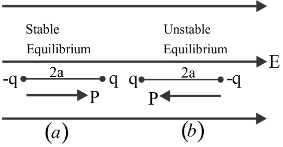
When $\theta = {180^o}$ i.e., dipole is placed opposite to electric field, it is said to be in unstable equilibrium.
Stable equilibrium Unstable equilibrium
$\tau = 0$ ${\tau _{\max }} = pE$ $\tau = 0$
$W = 0$ $W = pE$ ${W_{\max }} = 2pE$
${U_{\min }} = - pE$ $U = 0$ ${U_{\max }} = pE$
Gauss’s Law
1. Electric Flux
1.1 Definition
Electric flux is defined as proportional to number of field lines crossing or cutting any area of cross section in space.
'The number of field lines passing through perpendicular unit area will be prop ortional to the magnitude of Electric Field there" (Theory of Field Lines)
$\dfrac{{\text{N}}}{{{{\text{A}}_ \bot }}} \propto {\text{E}} \Rightarrow {\text{N}} \propto {{\text{E}}_ \bot }$
$\therefore \quad $ Electric Flux, ${\Phi _{{A_ \bot }}} = {\text{E}}{{\text{A}}_ \bot }$
As $\theta $ increases, flux through area A decreases. If we draw a vector of magnitude ${\text{A}}$ along the positive normal, it is called the area vector, $\vec A$ corresponding to the area $A$.
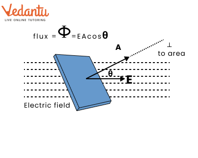
$\therefore \quad $ Electric Flux, ${\Phi _A} = {\text{EA}}\cos \theta = \overrightarrow {\text{E}} \cdot \overrightarrow {\text{A}} $
(Assuming Electric Field is uniform over whole area)
Note:
If Electric field is not constant over the area of cross section, then
$\Phi = \int_A {\overrightarrow {\text{E}} } \cdot {\text{d}}\overrightarrow {\text{A}} $
1.2 Unit and Dimension
Flux is a scalar quantity.
S.I. unit : (volt $ \times {\text{m}})$ or $\dfrac{{{\text{N}} \cdot {{\text{m}}^2}}}{{\text{C}}}$
It 's Dimensional formula: $\left( {{\text{M}}{{\text{L}}^3}\;{{\text{T}}^{ - 3}}\;{{\text{A}}^{ - 1}}} \right)$
1.3 Types of Flux
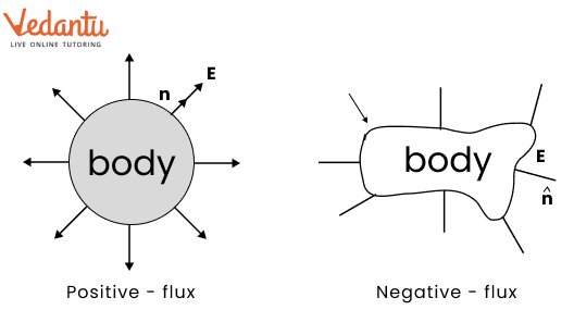
For a closed body outward flux is taken to be positive, while inward flux is taken to be negative.
2. Gauss's Law
2.1 Definition
According to Gauss's law, total electric flux through a closed surface enclosing a charge is $\dfrac{1}{{{\varepsilon _0}}}$ times the magnitude of the charge enclosed.
i.e., ${\phi _{{\text{not}}}} = \dfrac{1}{{{\varepsilon _0}}}\left( {{Q_{{\text{cc}}}}} \right)$
i.e., $\oint {\vec E} \cdot d\vec A = \dfrac{{{Q_{en}}}}{{{E_0}}}$.
Note:
Gauss's law is only applicable for a closed surface.
2.2 Gaussian Surface
The closed surface on which Gauss law is applicable is defined as a Gaussian surface.
Note:
Gaussian surface can be of any shape \& size, only condition is that it should be closed.
Gaussian surface is hypothetical in nature. It does not have a physical existence.
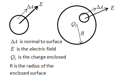
2.3 Deriving Gauss's Law from Coulomb's Law
Let’s take a spherical gaussian surface with charge '$ + Q$' kept at the centre.
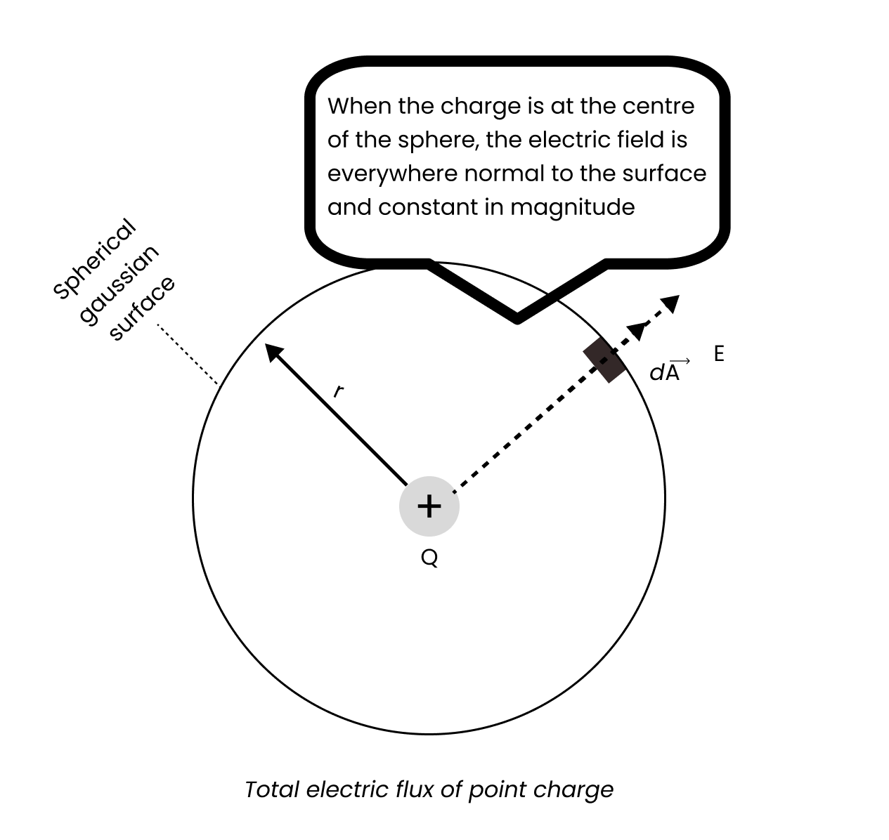
We know field lines for a +ve charge are always radially outward.
Angle between $d\vec A$ and $\vec E$ is zero.
${\text{E}} = \dfrac{{{\text{kQ}}}}{{{{\text{r}}^2}}} = \dfrac{{\text{Q}}}{{4\pi { \in _0}{{\text{r}}^2}}}$
(Image will be uploaded soon)
Hence Net flux $ = Q/{\varepsilon _0}$.
Although we derived gauss law for a spherical surface it is valid for any shape of gaussian surface and for any charge kept anywhere inside the surface.
2.4 Coulomb's Law from Gauss's Law
We choose an imaginary sphere (Gaussian surface) of radius ${\text{r}}$ centred on the charge $ + {\text{q}}$. Due to symmetry, ${\text{E}}$ must have the same magnitude at any point on the surface, and $\vec E$ points radially outward, parallel to $\overrightarrow {{\text{dA}}} $. Hence we write the integral in Gauss's law as:
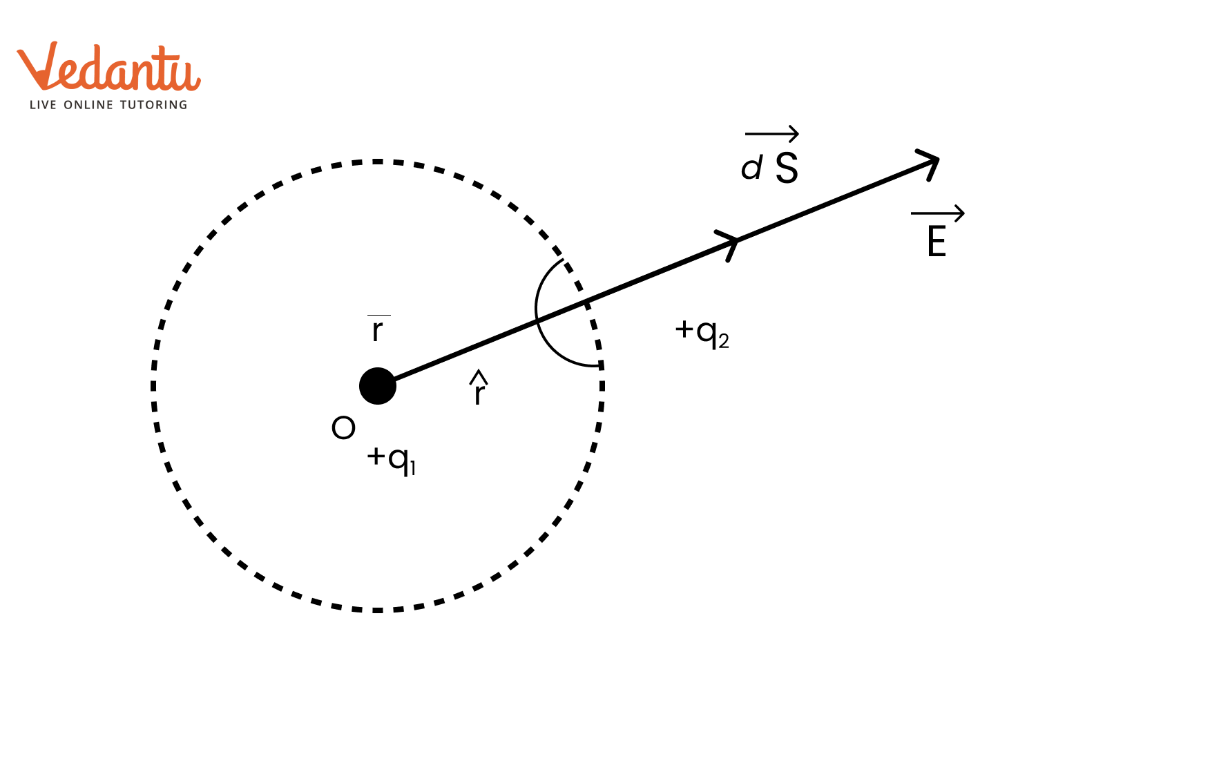
${\phi _{{\text{net }}}} = \oint {\vec E} \cdot \overrightarrow {dA} = \oint E dA = E\oint d A = E\left( {4\pi {r^2}} \right)$
${Q_{{\text{enclosed }}}} = q$
Thus, $E\left( {4\pi {r^2}} \right) = \dfrac{q}{{{\varepsilon _0}}}$ or $E = \dfrac{q}{{4\pi {\varepsilon _0}{r^2}}}$
From the definition of the electric field, the force on a point charge ${{\text{q}}_0}$ located at a distance ${\text{r}}$ from the charge q is ${\text{F}} = {{\text{q}}_0}{\text{E}}$. Therefore,
${\text{F}} = \dfrac{1}{{4\pi {\varepsilon _0}}}\dfrac{{{\text{q}}{{\text{q}}_0}}}{{{{\text{r}}^2}}}$
which is Coulomb's law.
3. Applications of Gauss's Law
Using Gauss's law to derive ‘E’ due to various charge distributions.
3.1 Electric Field Due to a Line Charge
Consider an infinite line which has a linear charge density $\lambda $. Using Gauss's law, let us find the electric field at a distance '${\text{r}}$' from the line charge.
The cylindrical symmetry tells us that the field strength will be the same at all points at a fixed distance $r$ from the line. Thus, if the charges are positive. The field lines are directed radially outwards, perpendicular to the line charge.
The appropriate choice of Gaussian surface is a cylinder of radius $r$ and length ${\text{L}}$. On the flat end faces, ${{\text{S}}_2}$ and ${{\text{S}}_3},\overrightarrow {\text{E}} $ is perpendicular ${\text{d}}\overline {\text{S}} $, which means flux is zero on them. On the curved surface ${S_1},\vec E$ is parallel to $d\bar S$, so that $\overrightarrow {\text{E}} \cdot \overrightarrow {{\text{dS}}} = {\text{EdS}}$. The charge enclosed by the cylinder is $Q = \lambda L$. Applying Gauss's law to the curved surface, we have
${\text{E}}\oint {{\text{dS}}} = {\text{E}}(2\pi {\text{rL}}) = \dfrac{{\lambda {\text{L}}}}{{{\varepsilon _0}}}{\text{ or E}} = \dfrac{\lambda }{{2\pi {\varepsilon _0}{\text{r}}}} = \dfrac{{{\text{2k\lambda }}}}{{\text{r}}}$
Note:
This is the field at a distance ${\text{r}}$ from the line. It is directed away from the line if the charge is positive and towards the line if the charge is negative.
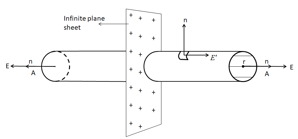
3.2 Electric Field Due to a Plane Sheet of Charge
Consider a large plane sheet of charge with surface charge density (charge per unit area) $\sigma $. We have to find the electric field ${\text{E}}$ at a point ${\text{P}}$ in front of the sheet.
Note:
If the charge is positive, the field is away from the plane.
To calculate the field ${\text{E}}$ at ${\text{P}}$. Choose a cylinder of area of cross-section A through the point P as the Gaussian surface. The flux due to the electric field of the plane sheet of charge passes only through the two circular caps of the cylinder.
According to Gauss law $\oint {\vec E} \cdot d\bar S = {q_{{\text{in }}}}/{\varepsilon _0}$
\[\mathop {\int {\overrightarrow E .\overline {dS} } }\limits_{{\text{I circular surface}}} + \mathop {\int {\overrightarrow E .\overline {dS} } }\limits_{{\text{II circular surface}}} + \mathop {\int {\overrightarrow E .\overrightarrow {dS} } }\limits_{{\text{cylindricalr surface}}} = \dfrac{{\sigma A}}{{{\varepsilon _0}}}\]
or ${\text{EA}} + {\text{EA}} + 0 = \dfrac{{\sigma {\text{A}}}}{{{\varepsilon _0}}}$
or $E = \dfrac{\sigma }{{2{\varepsilon _0}}}$
Note:
We see that the field is uniform and does not depend on the distance from the charge sheet. This is true as long as the sheet is large as compared to its distance from ${\text{P}}$.
3.3 Uniform Spherical Charge Distribution
3.3.1 Outside the Sphere
P is a point outside the sphere at a distance $r$ from the centre.
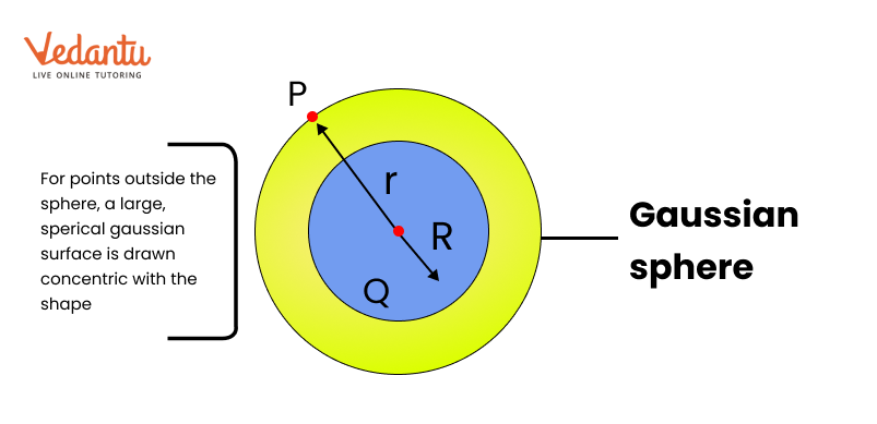
According to Gauss law, $\oint {\overrightarrow {\text{E}} } \cdot {\text{d}}\overrightarrow {\text{s}} = \dfrac{{\text{Q}}}{{{{\text{E}}_{\text{D}}}}}$ or ${\text{E}}\left( {4\pi {{\text{r}}^2}} \right) = \dfrac{{\text{Q}}}{{{\varepsilon _{\text{D}}}}}$
Electric field at P (Outside sphere)
${E_{{\text{out }}}} = \dfrac{1}{{4\pi {\varepsilon _0}}} \cdot \dfrac{Q}{{{r^2}}} = \dfrac{{\sigma {R^2}}}{{{\varepsilon _0}{r^2}}}$ and
${{\text{V}}_{{\text{out }}}} = - \int_\infty ^{\text{r}} {\overrightarrow {\text{E}} } {\text{d}}\overrightarrow {\text{r}} = \dfrac{1}{{4\pi {\varepsilon _0}}} \cdot \dfrac{{\text{Q}}}{{\text{r}}} = \dfrac{{\sigma {{\text{R}}^2}}}{{{\varepsilon _0}{\text{r}}}}$
Note:
${Q = 0 \times A}$
${ = \sigma \times 4\pi {R^2}}$
3.3.2 At the surface of sphere
At surface $r = R$
So, ${E_e} = \dfrac{1}{{4\pi {\varepsilon _0}}} \cdot \dfrac{Q}{{{R^2}}} = \dfrac{\sigma }{{{\varepsilon _0}}}$ and ${V_\varepsilon } = \dfrac{1}{{4\pi {\varepsilon _0}}} \cdot \dfrac{Q}{R} = \dfrac{{\sigma R}}{{{\varepsilon _0}}}$
3.3.3 Inside the Sphere
Inside the conducting charged sphere electric field is zero and potential remains constant everywhere and equals to the potential at the surface.
Class 12 Physics Chapter 1 Notes - Basic Subjective Questions
Section-A (1 Marks Questions)
1. Which orientation of an electric dipole in a uniform electric field would correspond to stable equilibrium?
Ans. When dipole moment vector is parallel to electric field $vector \vec{P}\parallel \vec{E}$ .
2. If the radius of the Gaussian surface enclosing a charge is halved, how does the electric flux through the Gaussian surface change?
Ans. Electric flux $\phi _{E}$ is given by
$\phi _{E}=\oint \vec{E}\cdot \vec{ds}=\dfrac{Q}{\varepsilon _{0}}$
where [Q is total charge inside the closed surface ∴ on changing the radius of sphere, the electric flux through the Gaussian surface remains same
3. Figure shows three point charges, +2q, -q and + 3q. Two charges +2q and -q are enclosed within a surface ‘S’. What is the electric flux due to this configuration through the surface ‘S’

Ans.Electric flux $=\oint_{s}^{}\vec{E}\cdot \vec{dS}$
According to Gauss’s’ law, $\phi =\oint_{s}^{}\vec{E}\cdot \vec{dS}=\dfrac{q_{1}}{\varepsilon _{0}}$ … where [q1 is the total charge enclosed by the surface S $\phi =\dfrac{2q-q}{\varepsilon _{0}}=\dfrac{q}{\varepsilon _{0}}\therefore$ electric flux, $\phi =\dfrac{q}{\varepsilon _{0}}$
4. What is the electric flux through a cube of side 1cm which encloses an electric dipole?
Ans. Zero because the net charge of an electric dipole (+ q and – q) is zero.
5. How does the electric flux due to a point charge enclosed by a spherical Gaussian surface get affected when its radius is increased?
Ans. The electric flux due to a point charge enclosed by a spherical gaussian surface remains ‘unaffected’ when its radius is increased.
Section – B (2 Marks Questions)
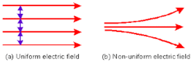
6. Differentiate between uniform electric field and non-uniform electric field.
Ans. Uniform electric field: In case of uniform electric field, the field lines are straight and equally spaced. Non- uniform electric field: in case of non uniform electric field, the field lines are not straight.
7. Is the electric field due to a charge configuration with total charge zero, necessarily zero? Justify.
Ans. No, it is not necessarily zero. If the electric field due to a charge configuration with total charge is zero because the electric field due to an electric dipole is non-zero.
8. Define the term electric dipole moment of a dipole. State its S.I. unit
Ans. τ = OE sin θ
If E = 1 unit, θ = 90°, then τ = P
Dipole moment may be defined as the torque acting on an electric dipole, placed perpendicular to a uniform electric dipole, placed perpendicular to a uniform electric field of unit strength. or Strength of the electric dipole is called the dipole moment.
$\left | \vec{P} \right | =q\left | 2a \right |$
∴ SI unit is Cm.
9. In which orientation, a dipole placed in a uniform electric field is in
(a) stable,
(b) unstable equilibrium?
Ans. For stable equilibrium, a dipole is placed parallel to the electric field.
For unstable equilibrium, a dipole is placed antiparallel to the electric field.
10. Define one coulomb. What is the SI unit of a charge?
Ans. One coulomb is the charge transferred in one second across a section of wire carrying current of one ampere.
SI unit of a charge is coulomb (C).
Important Formulas of Class 12 Chapter 1 Physics You Shouldn’t Miss!
Here are the important formulas for Class 12 Physics Chapter 1: Electric Charges and Fields that you shouldn’t miss:
1. Coulomb’s Law:
- The force between two point charges \( q_1 \) and \( q_2 \) separated by a distance \( r \) is given by:
\[F = k \cdot \frac{q_1 \cdot q_2}{r^2}\]
- Where \( k = \frac{1}{4\pi\epsilon_0} \) is the electrostatic constant, and \( \epsilon_0 \) is the permittivity of free space.
2. Electric Field Due to a Point Charge:
- The electric field \( E \) at a distance \( r \) from a point charge \( q \) is given by:
\[E = k \cdot \frac{q}{r^2}\]
3. Electric Field Due to a System of Charges:
- The resultant electric field at a point due to multiple charges is the vector sum of the electric fields due to each charge:
\[\mathbf{E} = \mathbf{E}_1 + \mathbf{E}_2 + \mathbf{E}_3 + \ldots\]
4. Electric Field on the Axis of a Dipole:
- The electric field at a point on the axial line of an electric dipole:
\[E_{\text{axial}} = \frac{1}{4\pi\epsilon_0} \cdot \frac{2p}{r^3}\]
- Where \( p = q \times 2a \) is the dipole moment and \( r \) is the distance from the center of the dipole.
5. Electric Field on the Equatorial Plane of a Dipole:
- The electric field at a point on the equatorial line of an electric dipole:
\[E_{\text{equatorial}} = \frac{1}{4\pi\epsilon_0} \cdot \frac{p}{r^3}\]
6. Electric Potential Due to a Point Charge:
- The electric potential \( V \) at a distance \( r \) from a point charge \( q \) is given by:
\[V = k \cdot \frac{q}{r}\]
7. Electric Potential Energy of a System of Two Charges:
- The potential energy \( U \) of a system of two point charges \( q_1 \) and \( q_2 \) separated by a distance \( r \):
\[U = k \cdot \frac{q_1 \cdot q_2}{r}\]
8. Gauss’s Law:
- The net electric flux \( \Phi_E \) through a closed surface is equal to the charge enclosed divided by the permittivity of free space:
\[\Phi_E = \oint \mathbf{E} \cdot d\mathbf{A} = \frac{q_{\text{enc}}}{\epsilon_0}\]
9. Electric Field Due to an Infinite Plane Sheet of Charge:
- The electric field due to an infinite plane sheet of charge with surface charge density \( \sigma \) is:
\[E = \frac{\sigma}{2\epsilon_0}\]
10. Electric Field Due to a Spherical Shell:
- Inside the shell: \( E = 0 \)
- On the surface: \( E = \frac{1}{4\pi\epsilon_0} \cdot \frac{Q}{R^2} \)
- Outside the shell: \( E = \frac{1}{4\pi\epsilon_0} \cdot \frac{Q}{r^2} \), where \( Q \) is the total charge and \( R \) is the radius of the shell.
Importance of Chapter 10 Electric Charges and Fields Class 12 Notes
Foundation for Advanced Topics: Electric Charges and Fields forms the basis for more advanced topics in mathematics and science, including physics and engineering. Mastering this chapter is essential for tackling these higher-level subjects.
Real-World Applications: Vectors are used in various real-world applications, such as in physics to describe forces and motion, and in computer graphics for modeling and animations. Knowing how to work with vectors is valuable in these fields.
Problem-Solving Skills: The concepts of vector addition, subtraction, and multiplication enhance problem-solving skills and mathematical reasoning, which are important for both academic and practical scenarios.
Exam Preparation: Electric Charges and Fields is a key topic in Class 12 exams. Detailed notes help you understand core concepts, practice solving different types of problems, and prepare effectively for tests and exams.
Conceptual Clarity: Comprehensive notes provide clear explanations and practical examples, helping you build a solid understanding of vectors and their properties, which is crucial for academic success.
Tips for Learning the Class 12 Physics Chapter 1 Electric Charges and Fields
Understand Basic Concepts: Begin by understanding the fundamental concepts of vectors, including their definition, representation, and basic operations. Grasping these basics is crucial for solving more complex problems.
Familiarise with Vector Operations: Learn how to perform vector addition, subtraction, and scalar multiplication. Practice these operations with different examples to build a solid foundation.
Learn Dot and Cross Products: Study the formulas and methods for calculating dot products and cross products. These are essential for solving many problems in Electric Charges and Fields.
Practice Vector Magnitudes and Directions: Understand how to find the magnitude and direction of a vector. Practice problems that involve calculating the length of vectors and using unit vectors.
Use Geometric Interpretations: Visualise vectors geometrically. Understanding how vectors interact in space can help you better grasp their properties and applications.
Conclusion
Understanding the concepts of Electric Charges and Fields is crucial for building a strong foundation in Physics. The Class 12 notes provided here offer detailed explanations, key formulas, and practical examples to help you understand this essential chapter thoroughly. By regularly reviewing these notes and practicing problem-solving, you can enhance your comprehension and perform confidently in your exams. Make the most of these resources to solidify your understanding and excel in your studies.
Related Study Materials for Class 12 Physics Chapter 10 Electric Charges and Fields
Students can also download additional study materials provided by Vedantu for Class 12 Physics Chapter 10 Electric Charges and Fields.
Chapter-wise Links for Class 12 Physics Notes PDF FREE Download
Related Study Materials Links for Class 12 Physics
Along with this, students can also download additional study materials provided by Vedantu for Physics Class 12–
FAQs on CBSE Notes Class 12 Physics Chapter 1 - Electric Charges and Fields - 2026-27
1. What are the key properties of electric charge that every Class 12 student should recall during quick revision?
Electric charges have essential properties such as quantization (they exist in discrete values as multiples of the elementary charge), conservation (total charge is unchanged in an isolated system), additivity (charges add algebraically), and transferability (charges can be moved from one object to another). Charges also produce electric and magnetic fields and are always associated with matter, but mass can exist without charge.
2. How does Coulomb's law define the interaction between two point charges, and what should be memorized for exam revision?
Coulomb's law states that the electrostatic force (F) between two point charges (q1 and q2) is directly proportional to the product of their magnitudes and inversely proportional to the square of the distance (r) between them. The formula is: F = k · (q1 · q2) / r2, where k = 1/(4πε0).
3. Why is the concept of electric field intensity fundamental for understanding electric charges and fields in Class 12?
Electric field intensity describes the force experienced by a unit positive charge placed at a specific point in space due to another charge. It is essential because it allows students to calculate how charges influence each other without direct contact and underpins many derivations and applications in Class 12 Physics.
4. Can you summarise the different methods of charging a body that should be revised before exams?
- By friction: Rubbing transfers electrons between two bodies.
- By conduction: A charged object touches an uncharged conductor, transferring charge.
- By induction: A charged object is brought near an uncharged object, causing redistribution of charges without direct contact.
5. What does the principle of superposition state, and how is it applied in problems involving multiple charges?
The superposition principle states that the net force or electric field on a charge caused by several other charges is the vector sum of the forces or fields exerted by each charge individually. This allows calculation of resultants in multi-charge systems by adding up all contributions using vector addition.
6. How do the properties of electric field lines assist in visualising and solving problems on Electric Charges and Fields?
- Field lines originate from positive and end at negative charges.
- The density of field lines indicates the strength of the field.
- Field lines never cross each other.
- Their direction shows the force on a positive test charge.
- Field lines help visualise uniformity, direction, and relative strengths in different regions, which aids in conceptual clarity and problem-solving.
7. What is Gauss's Law, and how does it simplify electrostatic calculations in Class 12 Physics?
Gauss's Law relates the total electric flux through a closed surface to the charge enclosed by that surface: ΦE = Qenclosed / ε0. It provides a shortcut for finding electric field in highly symmetric situations (such as spherical, cylindrical, or planar charge distributions), bypassing complex integration.
8. What is the significance of electric flux, and how does its value change with the size and shape of the Gaussian surface?
Electric flux is proportional to the number of electric field lines passing through a surface. For a closed surface enclosing a net charge, the flux depends only on the enclosed charge—not on the size or shape of the surface—thanks to Gauss's Law.
9. In which situations is the electric field inside a charged conductor zero, and what are the implications for potential?
Inside a charged conductor at electrostatic equilibrium, the electric field is always zero because free charges rearrange themselves on the surface to cancel any interior field. As a result, the potential is constant throughout the conductor and equal to the value at its surface.
10. How do you differentiate between a uniform and non-uniform electric field with reference to field lines and physical conditions?
- Uniform electric field: Field lines are straight, parallel, and equally spaced. Strength and direction are constant everywhere.
- Non-uniform electric field: Field lines are curved or unevenly spaced. Strength and/or direction varies from point to point.
11. What is the definition and physical meaning of the electric dipole moment, and how is it calculated?
The electric dipole moment (→p) is a vector quantity defined as the product of the magnitude of charge (q) and the distance separating the equal and opposite charges (2a). Formula: p = q × 2a. It quantifies the strength and orientation of a dipole.
12. What happens when an electric dipole is placed in a uniform electric field, and how are stable and unstable equilibrium determined?
A dipole in a uniform field experiences zero net force but a torque that tends to align it with the field.
- Stable equilibrium: Dipole moment is parallel to the field.
- Unstable equilibrium: Dipole moment is antiparallel to the field.
13. Is the electric field always zero if the total charge in a configuration is zero? Justify your answer for board revision.
No, the electric field is not necessarily zero even if the net charge is zero. For example, an electric dipole has zero total charge but creates a non-zero field in the surrounding region due to charge separation.
14. What critical formulas from Electric Charges and Fields should be prioritised during last-minute revision for Class 12 Physics?
- Coulomb's Law: F = k · (q1 · q2) / r2
- Electric Field by point charge: E = k · q / r2
- Field due to dipole axis: E = (1/4πε0) · (2p/r3)
- Electric Flux: Φ = E · A · cosθ
- Gauss's Law: ΦE = Qenclosed / ε0
15. How can understanding the concept of equilibrium of charges help solve advanced exam questions efficiently?
Recognising conditions for electrostatic equilibrium—where net force on each charge is zero—helps quickly determine positions, magnitudes, or directions required for balancing charges in complex setups, thus streamlining problem-solving in board exams.