Linear Programming Class 12 Notes: CBSE Maths Chapter 12

Linear Programming & Its Applications

• Linear Programming is a common optimization (maximisation or minimization) approach used in business and everyday life to find the maximum or minimum values necessary of a linear expression in order to meet a set of supplied linear constraints.

• It may entail determining the most profit, the lowest cost, or the least amount of resources used, among other things.

• Industry, commerce, management science, and other fields use it.

Linear Programming Problem and its Mathematical Formulation

Optimal value:

It refers to the Maximum or Minimum value of a linear function.

Objective Function:

• The function that needs to be improved (maximized/minimized)

• Linear function $\text{Z = ax + by }$, where $\text{a, b}$ are constants, which has to be maximised or minimized is called a linear objective function.

• For example, $\text{Z = 250x + 75y }$where variables $\text{x}$ and $\text{y}$ are called decision variables.
  
  

Linear Constraints:

• The objective function is to be optimised using a system of linear inequations/equations.

• In a linear programming issue, linear inequalities/equations or limitations on the variables are used.

• Also called Overriding Conditions or Constraints.

• The conditions $\text{x}\ge \text{0, y}\ge \text{0}$are called non-negative restrictions.
  
  

Non-Negative Restrictions:

All of the variables used to make decisions are assumed to have non-negative values.

Optimization Problem:

• A problem that seeks to maximize or minimize a linear function (say of two variables $\text{x}$ and $\text{y}$) subject to certain constraints as determined by a set of linear inequalities.

• Linear programming problems (LPP) are a special type of optimization problem.

Note:

• The term linear denotes that all of the mathematical relationships in the problem are linear.

• The term programming refers to the process of deciding on a specific program or course of action.
  
  

Mathematical Formulation of the Problem

• A general LPP can be stated as 

$\left( \text{Max / Min} \right)\text{ Z = }{{\text{c}}_{\text{1}}}{{\text{x}}_{\text{1}}}\text{+ }{{\text{c}}_{\text{2}}}{{\text{x}}_{\text{2}}}\text{+ }...\text{ + }{{\text{c}}_{\text{n}}}{{\text{x}}_{\text{n}}}$ 

(Objective function) subject to constraints and non-negative restrictions.

$\left\{ \begin{align} & {{\text{a}}_{\text{11}}}{{\text{x}}_{\text{1}}}\text{+ }{{\text{a}}_{\text{12}}}{{\text{x}}_{\text{2}}}\text{+ }...\text{ + }{{\text{a}}_{\text{1n}}}{{\text{x}}_{\text{n}}}\left( \le \text{ = }\ge  \right){{\text{b}}_{\text{1}}} \\  & {{\text{a}}_{\text{21}}}{{\text{x}}_{\text{1}}}\text{+ }{{\text{a}}_{\text{22}}}{{\text{x}}_{\text{2}}}\text{+ }...\text{ + }{{\text{a}}_{\text{2n}}}{{\text{x}}_{\text{n}}}\left( \le \text{ = }\ge  \right){{\text{b}}_{\text{2}}} \\  & \text{.} \\  & \text{.} \\  & \text{.} \\  & \text{.} \\  & {{\text{a}}_{\text{m1}}}{{\text{x}}_{\text{1}}}\text{+ }{{\text{a}}_{\text{m2}}}{{\text{x}}_{\text{2}}}\text{+ }...\text{ + }{{\text{a}}_{\text{mn}}}{{\text{x}}_{\text{n}}}\left( \le \text{ = }\ge  \right){{\text{b}}_{\text{m}}} \\  \end{align} \right\}$

• \[{{\text{x}}_{\text{1}}}\text{, }{{\text{x}}_{\text{2}}}\text{, }.....\text{, }{{\text{x}}_{\text{n}}}\ge 0\] where \[{{\text{a}}_{\text{11}}}\text{, }{{\text{a}}_{\text{12}}}\text{, }....\text{, }{{\text{a}}_{\text{mn}}}\];

• \[{{\text{b}}_{\text{1}}}\text{, }{{\text{b}}_{\text{2}}}\text{, }....\text{, }{{\text{b}}_{\text{m}}}\] and \[{{\text{c}}_{\text{1}}}\text{, }{{\text{c}}_{\text{2}}}\text{, }....\text{, }{{\text{c}}_{\text{n}}}\] are constants and

• \[{{\text{x}}_{\text{1}}}\text{, }{{\text{x}}_{\text{2}}}\text{, }.....\text{, }{{\text{x}}_{\text{n}}}\] are variables.
  
  

Graphical Method of Solving Linear Programming Problems

Terminologies

Solution of an LPP:

A set of values of the variables \[{{\text{x}}_{\text{1}}}\text{, }{{\text{x}}_{\text{2}}}\text{, }.....\text{, }{{\text{x}}_{\text{n}}}\] that satisfy the restrictions of an LPP.

Feasible Solution of an LPP:

• A set of values of the variables \[{{\text{x}}_{\text{1}}}\text{, }{{\text{x}}_{\text{2}}}\text{, }.....\text{, }{{\text{x}}_{\text{n}}}\] that satisfy the restrictions and non-negative restrictions of an LPP.

• Possible solutions to the restrictions are represented as points within and on the boundary of the feasible zone.
  
  

Feasible Region:

The common region determined by all the constraints including non-negative constraints \[\text{x, y}\ge \text{0}\] of a linear programming problem, is called the feasible region (or solution region) for the problem.

Feasible Choice:

Each point is in the feasible region.

Infeasible Region:

The region outside the feasible region.

Infeasible Solution:

Any point outside the feasible region.

Optimal Solution of an LPP:

A feasible solution of an LPP is said to be optimal (or optimum) if it also optimizes the objective function of the problem.

Graphical Solution of an LPP:

The solution of an LPP is obtained by the graphical method, that is by drawing the graphs corresponding to the constraints and the non-negative restrictions.

Unbounded Solution:

Such solutions exist if the value of the objective function can be increased or decreased forever.

Example: Graph the constraints stated as linear inequalities:

• $\text{5x + y }\le \text{ 100  }...\text{ }\left( 1 \right)$

• $\text{x + y }\le \text{ 60  }......\text{ }\left( 2 \right)$

• \[\text{x}\ge \text{ 0 }.................\text{ }\left( 3 \right)\]

• \[\text{y}\ge \text{ 0 }.................\text{ }\left( 4 \right)\]

Ans:

For Plotting the Equation (1),

• Let \[\text{x = 0}\]. Hence we get the point \[\text{y = 100}\]

• Let \[\text{y = 0}\]. Hence we get the point \[\text{x = }\dfrac{\text{100}}{5}=20\]

• The equation \[\left( 1 \right)\] is obtained by joining the points \[\left( 20,100 \right)\]

For Plotting the Equation \[\left( 2 \right)\],

• Let \[\text{x = 0}\]. Hence we get the point \[\text{y = 60}\]

• Let \[\text{y = 0}\]. Hence we get the point \[\text{x = 60}\]

• The equation \[\left( 2 \right)\] is obtained by joining the points \[\left( 60,60 \right)\]

• From Equation \[\left( 3 \right)\] and Equation \[\left( 4 \right)\], we know both \[\text{x}\] and \[\text{y}\] are more significant than \[\text{0}\].
  
  

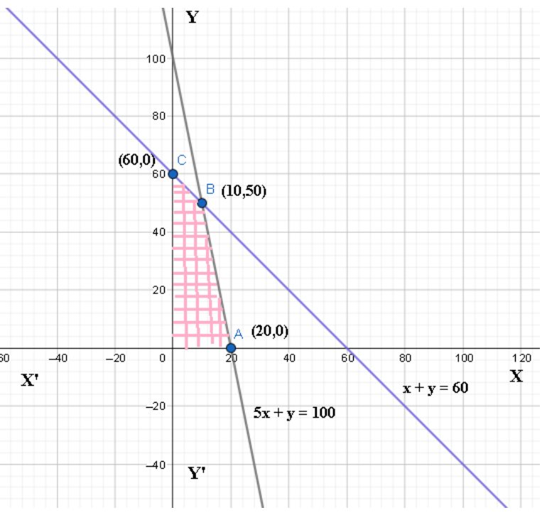
(Graph is drawn with the help of Geogebra and Paint)

From the graph above,

• Possible solutions to the constraints are represented by points within and on the edge of the feasible zone.

• Here, every point within and on the boundary of the feasible region $\text{OABC}$ represents a possible solution to the problem.

• For example, point $\left( 10,50 \right)$ is a feasible solution to the problem, and so are the points \[\left( 0,60 \right),\left( 20,0 \right)\], etc.

• Any point outside the possible region is called an infeasible solution. For example, point \[\left( 25,40 \right)\] is an infeasible solution to the problem.

• Now, we can see that every point in the feasible region $\text{OABC}$ satisfies all the constraints given in $\left( 1 \right)$to $\left( 4 \right)$. As there are endless points, it is unclear how to discover a position that yields the objective function's most significant value  $\text{z = 250x + 75y}$.

Theorem $\text{1}$

• Let $\text{R}$ be the feasible region (convex polygon) for a linear programming problem.  

• Let $\text{Z = ax + by }$ be the objective function.

• When the variables x and y are subject to constraints specified by linear inequalities, the optimal value Z (maximum or minimum) must occur at a corner point* (vertex) of the feasible region.
  
  

Theorem $\text{2}$ 

• Let $\text{R}$ be the feasible region for a linear programming problem.

• Let $\text{Z = ax + by }$ be the objective function.

• If an objective function $\text{R}$ is bounded, then the objective function $\text{Z}$ has both a maximum and a minimum value on $\text{R}$ and each of these occurs at a corner point (vertex) of $\text{R}$.
  
  

Remark:

The objective function may not have a maximum or minimum value if $\text{R}$ is unbounded. It must, however, occur at a corner point of $\text{R}$ if it exists.

A Graphical Approach to Solving a Linear Programming Issue

It can be solved by using below methods, they are as follows;

1. Corner point method

2. Iso-profit or Iso-cost method

Corner Point Method:

• Based on the principle of the extreme point theorem.

• Procedure to Solve an LPP Graphically by Corner Point Method

• Consider each constraint as an equation.

• Plot each equation on a graph, as each one will geometrically represent a straight line.

• The common region thus satisfies all the constraints, and the non-negative restrictions are called the feasible region. It is a convex polygon.

• Determine the vertices (corner points) of the convex polygon. These vertices are known as the feasible region's extreme points of corners.

• Find the objective function's values at each of the extreme points.

• The optimal solution of the given LPP is the point where the value of the objective function is optimum (maximum or minimum).
  
  

Isom-Profit or Iso-Cost Method:

Iso-profit or Iso-cost Method for Graphically Solving an LPP:

• Consider each constraint to be a mathematical equation.

• Draw each equation on a graph, as each one will represent a straight line geometrically.

• The polygonal region reached by meeting all constraints and non-negative limits is the feasible region, a convex set of all viable solutions of a given LPP.

• Determine the viable region's extreme points.

• Give the objective function $\text{Z}$ a handy value k and draw the matching straight line in the $\text{xy}$-plane.

• If the problem is maximization, draw parallel lines to $\text{Z = k}$ and find the line farthest from the origin and has at least one point in common with the viable zone.

• If the problem is of minimisation, then draw lines parallel to the line $\text{Z = k}$ that is closest to the origin and has minimum one point in common with the feasible zone. 

• The optimal solution of the given LPP is the common point so achieved.

Working Rule for Marking Feasible Region

Consider the constraint \[\text{ax + by}\le \text{c}\], where $\text{c  0}$.

• To begin, make a straight line \[\text{ax + by}=\text{c}\] y connecting any two points on it.

• Find two points that satisfy this equation as a starting point.

• This straight-line divides the \[\text{xy}\] -plane into two parts.

• The inequation \[\text{ax + by c}\] will represent that part of the \[\text{xy}\] -plane which lies to that side of the line \[\text{ax + by}=\text{c}\] in which the origin lies.

Again, consider the constraint \[\text{ax + by}\ge \text{c}\], where $\text{c  0}$.

• Draw the straight line \[\text{ax + by}=\text{c}\] by joining any two points on it.

• This straight-line divides the \[\text{xy}\]-plane into two parts.

• The inequation \[\text{ax + by}\ge \text{c}\] will represent that part of the \[\text{xy}\] -plane, which lies to that side of the line \[\text{ax + by}=\text{c}\] in which the origin does not lie.

Important Points to be Remembered

1. Basic Feasible Solution:

A fundamental solution that also meets the non-negativity constraints is known as a BFS.

2. Optimum Basic Feasible Solution:

A BFS is said to be optimum if it also optimizes (Max or min) the objective function.

Example: Solve the following linear programming problem graphically:

Maximize $\text{Z = 4x + y }...\text{ }\left( 1 \right)$

Subject to the constraints:

• \[\text{x + y }\le \text{ 50  }...\text{ }\left( 2 \right)\]

• $\text{3x + y }\le \text{ 90  }...\text{ }\left( 3 \right)$

• $\text{x}\ge \text{ 0 , y}\ge \text{ 0 }...\text{ }\left( 4 \right)$

Ans: For Plotting the Equation $\left( 2 \right)$ ,

• Let $\text{x = 0}$, Hence we get the point $\text{y = 50}$

• Let $\text{y = 0}$. Hence we get the point $\text{x = 50}$

• Equation $\left( 2 \right)$ is obtained by joining the points $\left( 50,50 \right)$

For Plotting the Equation $\left( 3 \right)$ ,

• Let $\text{x = 0}$. Hence we get the point $\text{y = 90}$

• Let $\text{y = 0}$. Hence we get the point $\text{x = 30}$

• The equation (3) is obtained by joining the points $\left( 30,90 \right)$

From Equation $\left( 4 \right)$, we know both $\text{x}$ and $\text{y}$ are greater than $\text{0}$.

As a result, the points are $\left( \text{0,0} \right)\text{, }\left( \text{50,50} \right)\text{, }\left( \text{0,50} \right)\text{, }\left( \text{30,0} \right)\text{, }\left( \text{30,90} \right)$.

The viable region in the graph is colored, as determined by the system of constraints $\left( 2 \right)$ to $\left( 4 \right)$.

The viable region \[\text{OAEC}\] is bounded, as shown below;

By replacing the vertices of the bounded region for the vertices of the bounded region, the maximum value of $\text{Z}$ may be determined using the Corner Point Method.

As a result, the highest value of $\text{Z}$ at the position is $\text{120}$ at the point $\left( 30,0 \right)$.

Example: Determine the minimum value of the objective function graphically.,

$\text{Z = -50x + 20y }...\text{ }\left( 1 \right)$

Subject to the constraints:

• $\text{2x - y }\ge \text{ -5 }...\text{ }\left( 2 \right)$

• $\text{3x + y }\ge \text{ 3 }...\text{ }\left( 3 \right)$

• $\text{2x - 3y }\le \text{ 12 }...\text{ }\left( 4 \right)$

• $\text{x}\ge \text{ 0 , y}\ge \text{ 0 }...\text{ }\left( 5 \right)$

Ans: We need to graph the feasible region of the system of inequalities $\left( 2 \right)$ to $\left( 5 \right)$. The visible shaded area is shown in the graph.

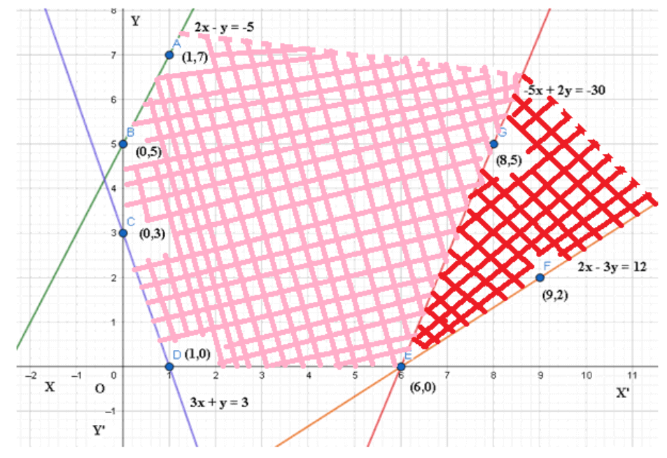
By Observation that the feasible region is unbounded.

At the corner points, we now examine $\text{Z}$ .

From this table, we found that $-300$ is the smallest value of $\text{Z}$ at the corner point $\left( 6,0 \right)$.

Since the region would have been bounded, this smallest value of $\text{Z}$ is the minimum value of $\text{Z}$  (Theorem $\left( 2 \right)$).

But here, we have seen that the feasible part is unbounded. 

Therefore, $-300$ may or may not be the minimum value of $\text{Z}$.

We use a graph to decide on this topic. 

$\text{-50x + 20y  -300}$ that is,

$\text{-5x + 2y  -30}$  (By dividing the above Equation by $\text{10}$)

And need to confirm whether the resulting open half-plane has points in common with the feasible region or not.

If it has common attributes, then $-300$ will not be the minimum value of $\text{Z}$ . Otherwise, $-300$ will be the minimum value of $\text{Z}$ .

As shown in the above graph, it has common points, and hence,

$\text{Z = -50x + 20y}$ has no minimum value subject to the given constraints.

General Features of Linear Programming Problems

1. A convex region is always the viable zone.

2. The vertex (corner) of the feasible region is where the objective function's maximum (or most minor) solution occurs.

3. If two corner points have the same maximum (or lowest) objective function value, then every point on the line segment connecting them has the same top (or minimum) value.

Different Types of Linear Programming Problems:

The following are some of the most crucial linear programming problems:

1. Manufacturing Problems:

When each product requires a fixed quantity of workforce, machine hours, labour hour per unit of product, warehouse space per unit of output, and so on, determine the number of units of various things that a company should manufacture and sell to optimise profit.

2. Diet Problems:

Determine the number of constituents/nutrients that should be included in a diet to keep the expense of the intended diet as low as possible while ensuring that each constituent/nutrient is present in a minimum amount.

3. Transportation problems:

Determine a transportation timetable to determine the most cost-effective method of moving a product from various plants/factories to multiple to keep the intended diet’s expense markets.

Revision Notes CBSE Class 12 Maths Notes Chapter 12 Linear Programming

What is Linear Programming

Linear programming can be defined as the method that can be used for optimizing various operations. This is done with the help of some constraints. Linear programming also consists of linear functions. Linear functions, in turn, are subjected to various constraints in the form of linear equations. These constraints can also be in the form of inequalities.

An important point to stress in these revision notes of Class 12 Maths Chapter 12 is that linear programming can also be used for finding the optimum resource utilization. Also, if we look at the term ‘linear programming,’ then you will realize that it is made from two words. These words are linear and programming.

The word ‘linear’ refers to the relationship that exists between various variables with degree one. On the other hand, the word programming refers to the process of selecting the best solution out of all alternatives.

Students who are going through these Class 12 Notes on Linear Programming should note that apart from mathematics, the concept of linear programming is also used in other fields. Some of those fields are manufacturing, business, economics, and telecommunication.

It would be best if you also remembered that linear programming is also known as linear optimization. It is also known by its abbreviated form, which is LP. Linear programming can also be used for calculating loss and profit.

According to various NCERT Class 12 Revision Notes Maths Chapter 12, there are different assumptions that are made while working with linear programming. And these assumptions are mentioned below.

• The linear function or the objective function has to be optimized

• The total number of constraints should be expressed in quantitative terms

• The relationship that exists between the objective function and the constraints should also be linear

It is vital for all students to be familiar with these assumptions before they practice questions related to the Maths Class 12 Chapter 12 Revision Notes.

Apart from the assumptions, there are also some essential components that are related to linear programming. Do you want to know what those components are? If yes, then go through the list that is mentioned below.

• Data

• Constraints

• Decision variables

• Objective functions

The topic of Class 12 Revision Notes Chapter 12 cannot be complete without talking about the vital characteristics of linear programming. So, this is precisely what we will discuss now.

There are many NCERT solutions Chapter 12 Class 12 Maths Revision Notes that state that there are five characteristics of a linear programming problem. These characteristics are:

Constraints

Constraints can be explained as the limitations that are imposed in a mathematical form. This is usually regarding the resource.

Objective Function

The objective function should always be specified in a quantitative way when it comes to a linear programming problem.

Linearity

Linearity can be described as the relationship that exists between two or more variables in a function. It must always be linear. This means that the degree of the variable should always be equal to one.

Finiteness

According to the Class 12 Maths Revision Notes Chapter 12, there should always be finite and infinite numbers of output and input. What we mean by this is that, if the function has infinite factors, then the optimal solution should not be feasible.

Non-Negativity

Non-negativity refers to the fact that the value of a variable should either be zero or position. A variable should not have a negative value.

The Applications of Linear Programming

There are many applications of linear programming. If we were to look at a real-time example, then it could be considering the limitations of materials and labour and finding the best production levels for the highest profit in various circumstances. This example is an integral part of optimization techniques, which is an important area of study in mathematics.

The applications of linear programming in other fields include solving problems related to design and manufacturing for shape optimization in the field of engineering. In the field of efficient manufacturing, linear programming helps in maximizing profits.

For the energy industry, linear programming plays a vital role by providing various methods for the optimization of the electric power system. Also, in transportation optimization, it can help with time efficiency and cost optimization.

Fun Facts about Linear Programming

Did you know that apart from optimizing various solutions, linear programming also solves many functional problems in operations analysis? These problems are represented as linear programming problems.

There are also some particular linear programming problems like multi-commodity flow queries and network flow queries. These problems are said to be important because these problems produce various research solutions on functional algorithms.

Linear Programming Class 12 Notes Maths - Basic Subjective Questions

Section–A (1 Mark Questions)

1. The feasible solution for a LPP is shown in following figure. Let Z=3x-4y be the objective function. Find where minimum of Z occurs.

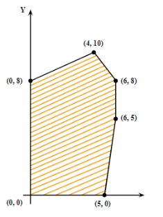
Ans. 

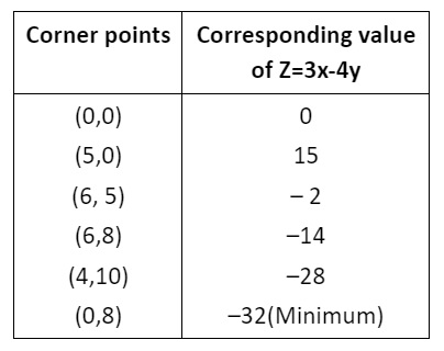
Hence, the minimum of Z  occurs at (0, 8) and its minimum value is -32. 

2. The feasible region for an LPP is shown in the following figure. Let F=3x-4y be the objective function. Then find the Maximum value of F.

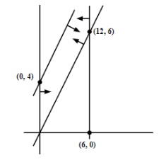
Ans. The feasible region as shown in the figure, has objective function F=3x-4y.

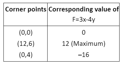
Hence, the maximum value of F is 12.

3. The feasible region for an LPP is shown in the following figure. Let F=3x-4y be the objective function. Then find the Minimum value of F.

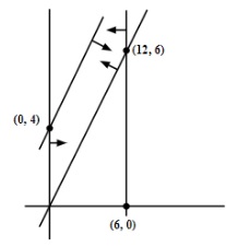
Ans. The feasible region as shown in the figure, has objective function F=3x-4y.

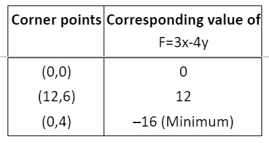
We have minimum value of F is –16 at   (0, 4).

4. Corner points of the feasible region for an LPP are (0, 2), (3, 0), (6, 0), (6, 8) and (0, 5). Let F=4x+6y be the objective function. Then find the value of Maximum of F- minimum of F.

Ans. 

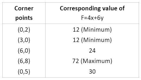
Maximum of F- Minimum of F=72-12=60. 

5. Corner points of the feasible region determined by the system of linear constraints are (0, 3), (1, 1) and (3, 0). Let Z=px+qy where pq>0. Then find the condition on p and q, so that the minimum of Z occurs at (3, 0) and (1, 1).

Ans. 

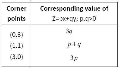
So, condition of p and q, so that the minimum of Z occurs at (3, 0) and (1, 1) is 

$q\;+q=3p$

$\Rightarrow 2p=q$

$\Rightarrow p=q/2$

Section–B (2 Marks Questions)

6. Maximize Z=3x+4y, subject to the constraints $x+y\leq 1,x\geq 0,y\geq 0$ .

Ans. We have to maximize Z=3x+4y,

Subject to the constraints $x+y\leq 1$ ; $x\geq 0$ and $y\geq 0$

All these inequalities are plotted as shown below:

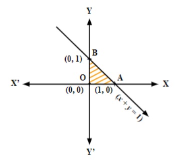
The shaded region shown in the figure as OAB is bounded and the coordinates of corner points O, A and B are (0, 0), (1, 0) and (0, 1), respectively.

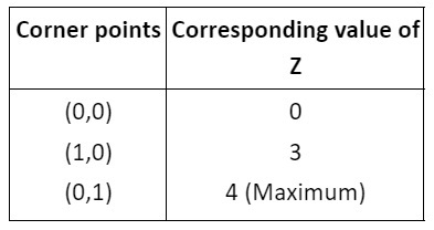
Hence, the maximum value of Z is 4 at  (0, 1).

7. Maximize the function Z=11x+7y subject to the constraints $x< 3,y\leq 2,x\geq 0$ and $y\geq 0$.

Ans. We have to maximize Z=11x+7y,

Subject to the constraints $x< 3,y\leq 2,x\geq 0$.

All these inequalities are plotted as shown below:

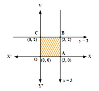
The shaded region OABC is bounded and the coordinates of corner points are (0, 0), (3, 0), (3, 2) and (0, 2), respectively.

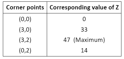
Hence, Z is maximum at (3, 2) and its maximum value is 47.

8. Minimize Z=13x-15y subject to the constraints $x+y\leq 7,2x-3y+6\geq 0,x\geq 0$ and $y\geq 0$ .

Ans. We have to minimize Z=13x-15y 

Subject to the constraints

$x+y\leq 7$

$2x-3y+6\geq 0$

$x\geq 0$ and $y\geq 0$

All these inequalities are plotted as shown below:

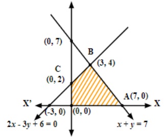
Shaded region shown as OABC is bounded and coordinates of its corner points are (0, 0), 

(7, 0), (3, 4) and (0, 2), respectively.

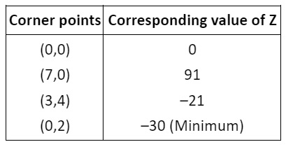
Hence, the minimum value of Z is –30 at (0, 2).

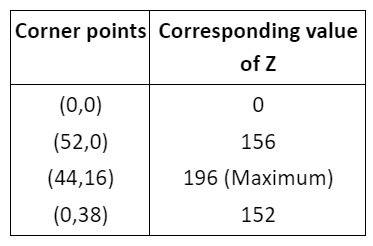
9. Determine the maximum value of Z=3x+4y, if the feasible region (shaded) for a LPP is shown in following figure.

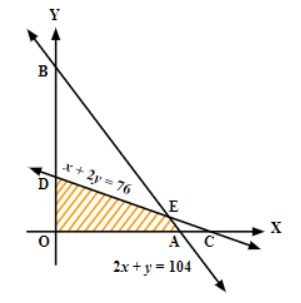
Ans. Two lines in graph are 2x+y=104 and 2x+4y=152

Solving the equations of two lines we have:

$\Rightarrow -3y=-48$

$\Rightarrow y=16 and x=44$

Thus, the point of intersection of two lines is E(44,16).

From the graph, corner points are O(0,0), A(52,0), E(44,16) and D(0,38). 

Also, given region is bounded.

Here, Z=3x+4y

Hence, Z at (44, 16) is maximum and its maximum value is 196.

10. Feasible region (shaded) for a LPP is shown in following figure. Maximize Z= 5+7y.

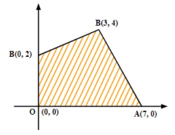
Ans. The shaded region is bounded and has coordinates of corner points as (0, 0), (7, 0), (3, 4) and (0, 2). Also, Z=5x+7y.

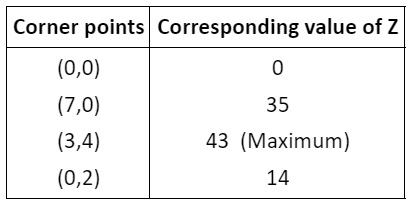
Hence, the maximum value of Z is 43 at  (3, 4).

11. The feasible region for a LPP is shown in following figure. Find the minimum value of Z = 11x+7y.

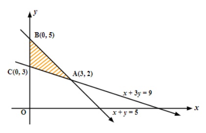
Ans. Lines x+3y=9 and x+y=5 intersect at (3, 2).

From the figure, it is clear that feasible region is bounded with corner points as (0, 3), (3, 2) and (0, 5).

Here, Z=11x+7y. 

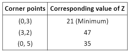
Hence, minimum value of Z is 21 at  (0, 3).

12. The feasible region for a LPP is shown in following figure. Find the maximum value of Z=11x+7y.

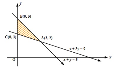
Ans. Lines x+3y=9 and x+y=5 intersect at (3, 2).

From the figure, it is clear that feasible region is bounded with corner points as (0, 3), (3, 2) and (0, 5).Here, Z= 11x+7y.

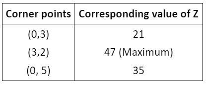
Hence, Z  is maximum at (3, 2) and its maximum value is 47.

13. The feasible region for a LPP is shown in the following figure. Evaluate Z=4x+y at each of the corner points of this region. Find the minimum value of Z if it exists.

Ans.  x+2y=4 and x+y=3 intersect at (2, 1)

From the figure the feasible region is the unbounded region with the corner points A(4,0), B(2,1) and C(0,3) Also, we have Z=4x+y 

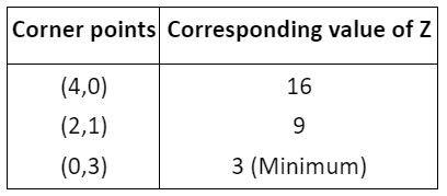
Here, 3 is the smallest value of Z at the corner point (0, 3). Now as the region is unbounded,

therefore 3 may or may not be the minimum value of Z.

To decide this issue, we graph the inequality $4x+y\leq 3$ and check that the resulting open half plane has no point in common with feasible region otherwise, Z has no minimum value. 

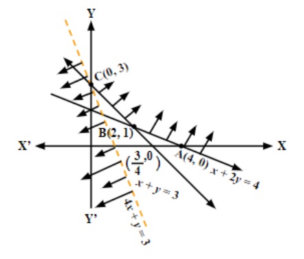
From the graph shown above, it is clear that there is no point in common with feasible region and hence Z has minimum value 3 at (0, 3). 

Important Formulas of Class 12 Maths Chapter 12 Linear Programming You Shouldn’t Miss!

Here are the important formulas and concepts for Class 12 Maths Chapter 12 Linear Programming that you shouldn't miss:

1. Objective Function:

- Maximize or Minimize $ Z = c_1 x_1 + c_2 x_2 $

- Where $ Z $ is the objective function, $ c_1 $ and $ c_2 $ are coefficients, and $ x_1 $ and $ x_2 $ are decision variables.

2. Constraints:

- Linear inequalities such as $ a_1 x_1 + a_2 x_2 \leq b $, $ a_1 x_1 + a_2 x_2 \geq b $, or $ a_1 x_1 + a_2 x_2 = b $

- Where $ a_1 $ and $ a_2 $ are coefficients, and $ b $ is the constraint value.

3. Feasible Region:

- The feasible region is the intersection of all constraint inequalities and represents all possible solutions that satisfy all constraints.

4. Graphical Method:

- Corner Point Method: Evaluate the objective function at each corner point of the feasible region to find the optimal solution.

- Intersection Points: Solve equations of boundary lines to find intersection points (corner points).

5. Slack and Surplus Variables:

- Slack Variable: Added to a ≤ constraint to convert it into an equation.

- Surplus Variable: Subtracted from a ≥ constraint to convert it into an equation.

6. Duality:

- Primal and Dual Problems: For every linear programming problem (primal), there is a corresponding dual problem. Solutions to both problems are related.

Importance of Chapter 12 Linear Programming Class 12 Notes PDF

1. Clear Understanding: They provide a structured explanation of linear programming concepts, including objective functions, constraints, and graphical methods, which are essential for mastering the topic.

2. Effective Revision: The PDF format allows for easy access and quick revision of key formulas, methods, and concepts, which is vital for exam preparation.

3. Visual Aids: Notes often include diagrams and graphical representations of feasible regions and constraints, enhancing comprehension of complex topics.

4. Problem-Solving Techniques: The notes cover various problem-solving techniques, such as the graphical method, helping students apply these methods effectively in different scenarios.

5. Practice and Application: With examples and practice problems included, the notes help students apply theoretical concepts to practical problems, improving problem-solving skills.

6. Exam Preparation: Comprehensive and well-organized notes ensure that students are well-prepared for exams by covering all necessary aspects of linear programming, leading to better performance.

Tips for Learning the Class 12 Maths Chapter 12 Linear Programming

1. Understand Key Concepts: Familiarise yourself with the basic concepts of linear programming, such as the objective function, constraints, feasible region, and optimal solution. A solid grasp of these fundamentals is essential.

2. Master Formulas and Methods: Memorise important formulas and methods, including the graphical method. Practice applying these formulas to different problems to reinforce your understanding.

3. Practice Graphical Method: Draw the feasible region by plotting constraints on a graph. Identify corner points and evaluate the objective function at these points to find the optimal solution.

4. Solve Example Problems: Work through various example problems and past exam questions. This will help you understand how to apply concepts and methods to different types of linear programming problems.

5. Use Visual Aids: Utilise diagrams and graphical representations to visualise constraints, feasible regions, and solutions. This can make complex concepts easier to understand.

Conclusion

Mastering Class 12 Maths Chapter 12 Linear Programming is essential for understanding how to solve optimisation problems. By grasping key concepts, practising methods like the graphical approaches, and using visual aids, you can effectively tackle problems and prepare for exams. Regular review, practice, and discussion with peers will reinforce your learning and build confidence. With these strategies, you'll be well-equipped to handle linear programming questions and succeed in your studies.

Related Study Materials for Class 12 Maths Chapter 12 Linear Programming

Chapter-wise Revision Notes Links for Class 12 Maths

Important Study Materials for Class 12 Maths