


Physics Notes for Chapter 5 Magnetism and Matter Class 12 - FREE PDF Download


Section-A (1 Marks Questions)
1. The susceptibility of a magnetic material is 1.9 × 10⁻⁵. Name the type of magnetic materials it represents.
Ans. Paramagnetic Substances.
2. Where on the surface of Earth is the angle of dip zero?
Ans. At the magnetic equator, the angle of dip is 0°.
3. Where on the surface of Earth is the horizontal component of Earth’s magnetic field zero?
Ans. At poles of Earth the horizontal component of Earth’s magnetic field is zero.
4. What is the magnetic dipole moment associated with an electron due to its orbital motion in the first orbit of H-atom known as?
Ans. Bohr magneton.
5. What type of magnetic material is used in making permanent magnets?
Ans. Material having high coercivity and high retentivity is used in making permanent magnets.
Section – B (2 Marks Questions)
6. Magnetic field arises due to charges in motion. Can a system have magnetic moments even though its net charge is zero?
Ans. Yes. The average of the charge in the system may be zero. Yet, the mean of the magnetic moments due to various current loops may not be zero. In paramagnetic material, the atoms have a net dipole moment though their net charge is zero.
7. How does the (i) pole strength and (ii) magnetic moment of each part of a bar magnet change if it is cut into two equal pieces along its length?
Ans.
(i) The pole strength becomes half.
(ii) The magnetic magnet becomes half.
8. What is the angle of dip at a place? What is the angle of dip at a place where the horizontal and vertical components of the earth’s magnetic field are equal?
Ans. The angle of dip is the angle made by the earth's total magnetic field (denoted as B) with the horizontal direction in the magnetic meridian, known as the angle of dip (δ) at any place Angle of dip is 45°.
9. Which physical quantity has the unit Wb/m2? Is it a scalar or a vector quantity?
Ans. Magnetic field. It is a vector quantity.
10. Derive an expression for the potential energy of a magnetic dipole in a uniform magnetic field.
Ans. Torque experienced by a magnetic dipole placed in a uniform magnetic field,
$\tau =mB\;sin\theta\left [ since\vec{\tau }=\vec{m}\times \vec{B} \right ]$
The magnetic potential energy Um can be given by,
$u_{m}=\int \tau (\theta )d\theta$
$=\int mB\;sin\;\theta d\theta$
$=-mB\;cos\;\theta$
or, $u_{m}=-\vec{m}\cdot \vec{B}$
PDF Summary - Class 12 Physics Magnetism and Matter Notes (Chapter 5)
1. Magnetic Field and Force
Magnetic Field is an area around the magnet where material or a charge particle experiences the magnetic force.
Magnetic force is the attraction or the repulsive force that arises between the charged particle when placed close to each other.
Now, consider a positive charge $q$ moving in a uniform magnetic field $\overrightarrow B $ , with a velocity $\overrightarrow v $.
Let the angle between $\overrightarrow v $ and $\overrightarrow B $ be θ.
\[\overrightarrow F = qBv\sin \theta = {180^ \circ } \]
\[\vec {F_B}=q\left ( \vec v\times\vec B \right )\]
\[If\:{\text{ }}\theta = {\text{ }}90^\circ ,{\text{ }}then{\text{ }}sin{\text{ }}\theta = {\text{ }}1 \]
\[v{\text{ }}cos{\text{ }}\theta {\text{ }}\left( { = {\text{ }}{v_1}{\text{ }}} \right) \]
\[v = 0 \]
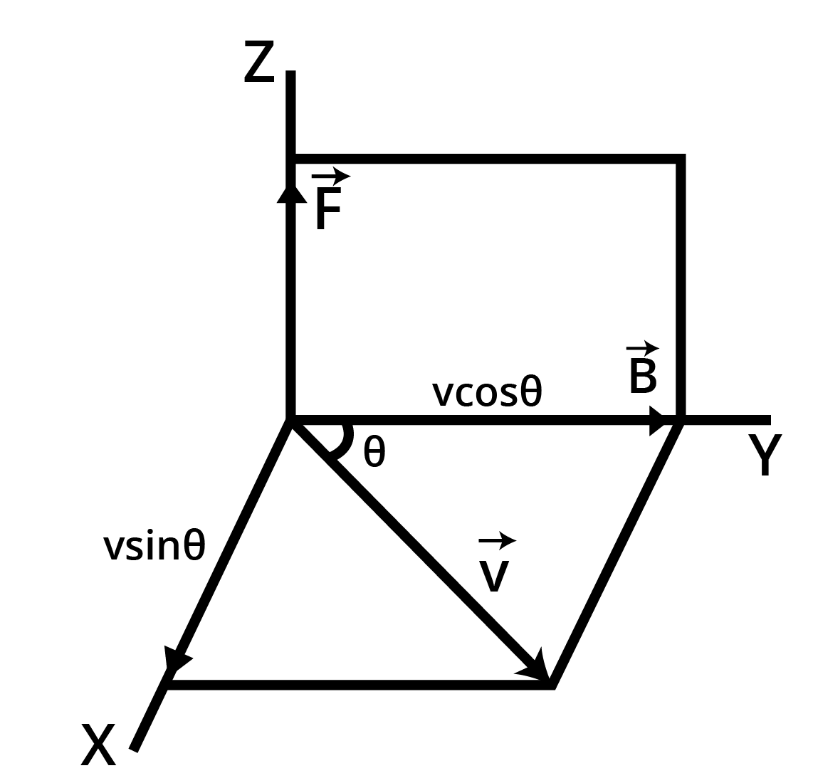
Diagram Showing the Direction Of Force, Magnetic Field and Motion of Charged Particles.
The magnitude of force $F$ experienced by the moving charge is directly proportional to the magnitude of the charge i.e. $F \propto q$
The magnitude of force $F$ is directly proportional to the component of velocity acting perpendicular to the direction of the magnetic field, i.e. \[F \propto v\sin \theta \]
The magnitude of force $F$ is directly proportional to the magnitude of the magnetic field applied i.e., \[F \propto B\] Combining the above factors, we get \[F \propto qBv\sin \theta \] or\[F = kqBv\sin \theta \] where k is a constant of proportionality. Its value is found to be one i.e. \[k = 1\].
\[\overrightarrow F = qBv\sin \theta \] …(1)
\[\overrightarrow F = \overrightarrow q (\overrightarrow v \times \overrightarrow B )\] …(2)
The direction of \[\overrightarrow F \] is same as the direction of \[(\overrightarrow v \times \overrightarrow B )\] , which is perpendicular to the plane containing \[\overrightarrow v \] and \[\overrightarrow B \]. Its direction is given by Right-handed-Screw Rule or Right-Hand Rule.
If \[\overrightarrow v \] and \[\overrightarrow B \] are in the plane of the paper, then according to Right-Hand Rule, the direction of \[\overrightarrow F \] on the positively charged particle will be perpendicular to the plane of paper upwards as shown in the figure and on the negatively charged particle will be perpendicular to the plane of paper downwards as shown in the figure.
Diagram Showing the Direction of Force, Magnetic Field and Motion of Charged Particles.
Definition of \[\overrightarrow B \]:
\[If{\text{ }}v{\text{ }} = {\text{ }}1,{\text{ }}q{\text{ }} = {\text{ }}1{\text{ }}and{\text{ }}sin{\text{ }}\theta {\text{ }} = {\text{ }}1{\text{ }}or{\text{ }}\theta = {\text{ }}90^\circ ,{\text{ }}then{\text{ }}from{\text{ }}\left( 1 \right),{\text{ }}F{\text{ }} = {\text{ }}1{\text{ }} \times {\text{ }}1{\text{ }} \times {\text{ }}B{\text{ }} \times {\text{ }}1{\text{ }} = {\text{ }}B.\]
The force experienced by a unit charge travelling with a unit velocity perpendicular to the direction of magnetic field induction at a place in the magnetic field is equal to the force experienced by a unit charge moving with a unit velocity perpendicular to the direction of magnetic field induction at that moment in time.
Special Cases:
Case-1 :
\[If{\text{ }}\theta {\text{ }} = {\text{ }}0^\circ {\text{ }}or{\text{ }}180^\circ ,{\text{ }}then{\text{ }}sin{\text{ }}\theta = {\text{ }}0.\]
\[\therefore\] From (1),
\[F{\text{ }} = {\text{ }}qv{\text{ }}B{\text{ }}\left( 0 \right){\text{ }} = {\text{ }}0.\]
That means, a charged particle moving along or opposite to the direction of magnetic field, does not experience any force.
Case-2 :
\[If{\text{ }}v{\text{ }} = {\text{ }}0\], then
\[F = {\text{ }}0.\]
That means, if a charged particle is at rest in a magnetic field, it experiences no force.
Case-3 :
\[If{\text{ }}\theta = {\text{ }}90^\circ ,{\text{ }}then{\text{ }}sin{\text{ }}\theta = {\text{ }}1\], then
\[\overrightarrow F = qBv\]
Note, SI unit of \[\overrightarrow B \] is tesla (\[T\]) or \[Weber/{(metre)^2}\] i.e. (\[Wb/{m^2}\] ) or \[Ns{\text{ }}{C^{--1}}{\text{ }}{m^{--1}}\].
Therefore, the magnetic field inducted at a point is said to be one tesla, if a charge of one coulomb while moving at right angle to a magnetic field, with a velocity of \[1{\text{ }}m{s^{--1}}\]experiences a force of \[1N\], at that point.
\[{\text{Dimensions of B}} = \dfrac{{{\text{ML}}{{\text{T}}^{ - 2}}}}{{{\text{AT}}\left( {{\text{L}}{{\text{T}}^{ - 1}}} \right)}} = \left. {{\text{M}}{{\text{A}}^{ - 1}}{{\text{T}}^{ - 2}}} \right]\]
2. Lorentz Force
Lorentz force is the force experienced by a charged particle travelling in space where both electric and magnetic fields exist.
Force due to electric field. When a charged particle carrying charge \[ + q\]is subjected to an electric field of strength \[\overrightarrow E \], it experiences a force given by:- \[{\overrightarrow F _e}{\text{ = }}\overrightarrow q \overrightarrow E {\text{ }}\] …(5)
whose direction is the same as that of \[\overrightarrow E \] .
Force Due to Magnetic Field. If the charged particle is moving in a magnetic field \[\overrightarrow B \], with a velocity \[\overrightarrow v \] it experiences a force given by:- \[\overrightarrow {{F_B}} = \overrightarrow q (\overrightarrow v \times \overrightarrow B )\] …(6)
The direction of this force is in the direction of \[(\overrightarrow v \times \overrightarrow B )\] i.e. perpendicular to the plane containing \[\overrightarrow v \]and \[\overrightarrow B \]and is directed as given by Right hand screw rule.
The total force experienced by the charged particle Due to both the electric and magnetic fields will be given by:-
\[\vec{F_e}+\vec{F_m}\:=\:q\vec{E}+q\left ( \vec v\:\times\:\vec B \right )=q\left ( \vec E\:+\:\left ( \vec v\times\vec B \right ) \right )\]
Special Cases:-
Case I:
When \[\overrightarrow v \], \[\overrightarrow E \] and \[\overrightarrow B \], all the three are collinear.
The magnetic force on the charged particle is zero since it is travelling parallel or antiparallel to the fields. The electric force on the charged particle will produce acceleration \[\vec a = \dfrac{q{\vec E}}{{\text{m}}}\] along the direction of electrical field. As a result, there will be a change in the speed of charged particles along the direction of the field.
So there will be no change in the direction of motion of the charged particle but, the speed, velocity, momentum and kinetic energy of charged particle will change.
Case II:
When \[\overrightarrow v \], \[\overrightarrow E \] and \[\overrightarrow B \] are mutually perpendicular to each other.
If \[\overrightarrow E \]and \[\overrightarrow B \] are such that \[\vec F\:=\vec {F_e}+\vec {F_m}= 0\], then acceleration in the particle,\[\vec a = \dfrac{{\vec F}}{m} = 0\]. That means the particle will pass through the fields without any change in its velocity. Here
\[{F_e}{\text{ }} = {\text{ }}{F_m}{\text{ }}\]so \[{\text{qE}} = {\text{q}} \vee {\text{B}}\] or
\[{\text{v}} = {\text{E}}/{\text{B}}\].
3. Motion of a Charged Particle in a Uniform Magnetic Field
Suppose a particle of mass \[m\] and charge \[q\], entering a uniform magnetic field induction \[\overrightarrow B \], \[with{\text{ }}velocity{\text{ }}\overrightarrow v \] making an angle \[\theta \] with the direction of magnetic field acting in the plane of paper as shown in figure:-
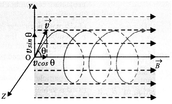
Motion of A Charged Particle in A Uniform Magnetic Field
Resolving \[\overrightarrow v \] into two rectangular components: \[v{\text{ }}cos{\text{ }}\theta {\text{ }}\left( { = {\text{ }}{v_1}{\text{ }}} \right)\] and \[v{\text{ }}sin{\text{ }}\theta {\text{ }}\left( { = {\text{ }}{v_2}{\text{ }}} \right)\]
Now, component velocity \[{v_2}\] , the force acting on the charged particle due to magnetic field is:-
\[\vec F = q\left ( \vec {v_2}\times\vec B \right )\]
\[{{\text{F}} =q\left | \vec {v_2}\times\vec B \right | = {\text{q}}{{\text{v}}_2}{\text{B}}\sin {{90}^ \circ } = {\text{q}}({\text{v}}\sin \theta ){\text{B}}}\]
As this force is to remain always perpendicular to \[{v_2}\] it does not perform any work and hence cannot change the magnitude of velocity \[{v_2}\].
It changes only the direction of motion. Due to it, the charged particle moves in a circular path in the magnetic field as shown in the figure:
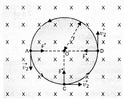
Diagram Showing the Circular Path Described By A Charged Particle in A Uniform Magnetic Field.
The magnetic field is depicted perpendicular to the plane of the paper, pointing inwards, and the particle is travelling in that plane. When the particle is at locations A, C, and D, the magnetic force on the particle will be directed along with AO, CO, and DO, respectively, i.e., towards the circular path's centre O.
The force F on the charged particle due to magnetic field provides the required centripetal force = \[\dfrac{{m{v^2}}}{r}\]
necessary for motion along a circular path of radius r.
\[\therefore \quad {\text{Bq}}{{\text{v}}_2} = \dfrac {m{{v_2}^2}}{r}\] \[{\text{or}}\:{{\text{v}}_2} = \dfrac {\text{Bqr}}{\text{m}}\]
\[{\text{or}}\quad v\sin \theta = {\text{Bqr}}/{\text{m}}\] ….(2)
The angular velocity of rotation of the particle in magnetic field will be:-
\[\omega = \dfrac{{{\text{V}}\sin \theta }}{{\text{r}}} = \dfrac{{{\text{Bqr}}}}{{{\text{mr}}}} = \dfrac{{{\text{Bq}}}}{{\text{m}}}\]
The frequency of rotation of the particle in magnetic field will be:-
\[{\text{v}} = \dfrac{\omega }{{2\pi }} = \dfrac{{{\text{Bq}}}}{{2\pi {\text{m}}}}\] …(3)
The time period of revolution of the particle in the magnetic field will be:-
\[{\text{T}} = \dfrac{1}{{\text{V}}} = \dfrac{{2\pi {\text{m}}}}{{{\text{Bq}}}}\] …(4)
We can see from (3) and (4) that v and T are independent of the particle's velocity v. It indicates that at a given position, all charged particles with the same particular charge (mass/charge) but moving at different velocities will complete their circular trajectories at the same time due to component velocities perpendicular to the magnetic fields.
For component velocity \[v{\text{ }}cos{\text{ }}\theta {\text{ }}\left( { = {\text{ }}{v_1}{\text{ }}} \right)\] there will be no force on the charged particle in the magnetic field, because the angle between \[{v_1}\] and \[\overrightarrow B \]is zero. As a result, the charged particle moves at a constant speed v cos in the direction of the magnetic field.
As a result of the combined effect of the two component velocities, the charged particle in a magnetic field will traverse both a linear and a circular course, i.e. the charged particle's path will be helical, with its axis parallel to the magnetic field direction, as shown in figure.
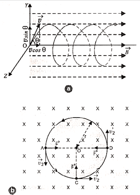
Charge Particle Describing A Helical Path in Uniform Magnetic Field.
The linear distance covered by the charged particle in the magnetic field in time equal to one revolution of its circular path (known as pitch of helix) will be:-
\[{\text{d}} = {{\text{v}}_1}{\text{T}} = {\text{v}}\cos \theta \dfrac{{2\pi {\text{m}}}}{{{\text{Bq}}}}\] .
Important Points
If a charged particle having charge \[\overrightarrow q \] is at rest in a magnetic field \[\overrightarrow B \], it experiences no force; as \[v = 0\]and \[\overrightarrow F = qBv\sin \theta = 0\].
If charged particle is moving parallel to the direction of \[\overrightarrow B \], it also does not experience any force because angle \[\theta \]between \[\overrightarrow v \]and \[\overrightarrow B \]is 0° or 180° and sin \[{0^ \circ }\] = sin \[{180^ \circ }\] = \[0\]. Therefore, the charged particle in this situation will continue moving along the same path with the same velocity.
If charged particle is moving perpendicular to the direction of \[\overrightarrow B \], it experiences a maximum force which acts perpendicular to the direction \[\overrightarrow B \]as well as \[\overrightarrow v \]. Hence this force will provide the required centripetal force and the charged particle will describe a circular path in the magnetic field of radius r, given by \[\dfrac{{{\text{m}}{{\text{v}}^2}}}{{\text{r}}} = {\text{Bqv}}\] .
4. Motion in Combined Electron and Magnetic Fields
4.1 Velocity Filter
A velocity filter is an arrangement of cross electric and magnetic fields in a region that allows us to choose charged particles with a specific velocity from a beam, regardless of their mass and charge.
A velocity selector is made up of two slits, $S_1$ and $S_2$, that are held parallel to each other and share a common axis. Uniform electric and magnetic fields are applied perpendicular to each other and to the axis of the slits in the region between the slits, as shown in the figure. After passing through slit $S_1$, a beam of charged particles of various charges and masses enters the region of the crossed electric field $\overrightarrow E $and magnetic field $\overrightarrow B $, each particle experiences a force due to these fields. Regardless of mass or charge, the force exerted on each particle by the electric field ($q\overrightarrow E $) is equal to and opposite to the force due to magnetic field $qvB$.
\[qE = q \vee B{\text{or}}v = E/B\].
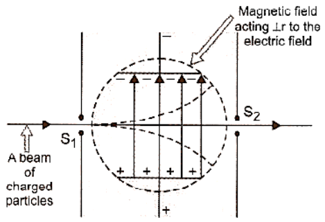
Velocity Filter
\[\overrightarrow {nBA/k} \]
\[\overrightarrow {{F_2}} \]
\[nBA/k \]
Such particles will pass through the slit S2 unaltered and filtered out of the zone. As a result, even if the charge and mass of the particles entering from slit S2 vary, they will all have the same velocity. In a mass spectrograph, the velocity filter is used to determine the mass and specific charge (charge/mass) of a charged particle.
4.2 Cyclotron
A cyclotron is a device developed by Lawrence and Livingstone by which positively charged particles like proton, deuteron, alpha particle etc. can be accelerated.
Principle. The working of the cyclotron is based on the fact that a positively charged particle can be accelerated to sufficiently high energy with the help of smaller values of the oscillating electric field by making it cross the same electric field time and again with the use of strong magnetic field.
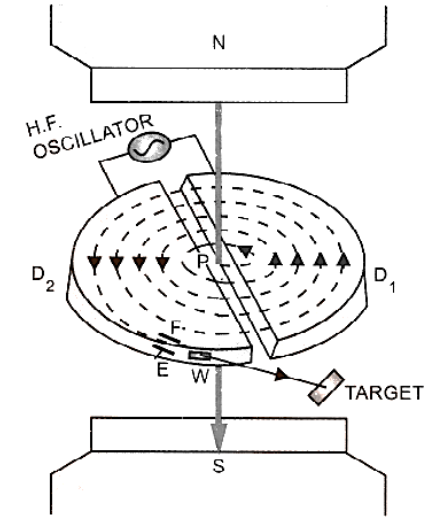
Construction:
It consists of two $D$-shaped hollow evacuated metal chambers $D_1$ and $D_2$ called the dees. These dees are placed horizontally with their diametric edges parallel and slightly separated from each other. The dees are connected to a high-frequency oscillator which can produce a potential difference of the order of $104V$ at frequency $ \approx {10^7}Hz$. The two dees are enclosed in an evacuated steel box and are well insulated from it. The box is placed in a strong magnetic field produced by two pole pieces of strong electromagnets $N, S$. The magnetic field is perpendicular to the plane of the dees. $P$ is a place of ionic source or positively charged particle figure.
Working and Theory:
At P, the positive ion that will be accelerated is created. Assume D1 is at a negative potential and D2 is at a positive potential at that time. As a result, the ion will accelerate toward D1. The ion will be in a field-free space after it enters D1. As a result, in D1, it moves at a constant speed of v. The ion, however, will trace a circular path of radius r due to a perpendicular magnetic field of intensity B in $D_1$, given by:
\[{\text{Bqv}} = \dfrac{{{\text{m}}{{\text{v}}^2}}}{{\text{r}}}\] .
\[\therefore \quad {\text{r}} = \dfrac{{{\text{mv}}}}{{{\text{Bq}}}}\]
Time taken by ion to describe a semi-circular path is given by,
${\text{t}} = \dfrac{{\pi {\text{r}}}}{{\text{v}}} = \dfrac{{\pi {\text{m}}}}{{{\text{Bq}}}} = \dfrac{\pi }{{{\text{B}}({\text{q}}/{\text{m}})}} = {\text{a}}$(constant)
This time is independent of both the speed of the ion and the radius of the circular path. If the time it takes for the positive ion to describe a semicircular path is equal to the time it takes for the electric oscillator's half-cycle to complete, then, as the ion enters the space between the two dees, it causes the polarity of the two dees has been switched, i.e. D1 is now D2 gets more favourable D1 and D2 negative. The positive ion is then accelerated in the direction of D2, it then moves on to D2 with a higher rate that remains D2's constant. The ion will be used to describe a semicircular route. Due to the perpendicular magnetic field, the radius is larger and will arrive between the two dees exactly at the same time. The polarity of the two dees is flipped for a brief moment. As a result, the positive ion will continue to accelerate every time it enters the space between the dees, describing a circular route of the increasing radius with increasing speed until it reaches sufficiently high energy. By providing an electric field across the deflecting plates E and F, the accelerated ion can be evacuated from the dees from window W.
Maximum Energy of Positive Ion:
Let ${v_0},{r_0} = $ maximum velocity and maximum radius of the circular path followed by the positive ion in cyclotron.
Then \[\dfrac{{{\text{mv}}_0^2}}{{{{\text{r}}_0}}} = {\text{Bq}}{{\text{v}}_0}{\text{or}}{{\text{v}}_0} = \dfrac{{{\text{Bq}}{{\text{r}}_0}}}{{\text{m}}}\]
\[\therefore\:{\text{Max}}{\text{. K}}{\text{.E}}{\text{.}} = \dfrac{1}{2}mv_0^2 = \dfrac{1}{2}m{\left( {\dfrac{{Bq{r_0}}}{m}} \right)^2} = \dfrac{{{B^2}{q^2}r_0^2}}{{2m}}\] .
Cyclotron Frequency:
If T is the time period of oscillating electric field then, \[{\text{T}} = 2{\text{t}} = 2\pi {\text{m}}/{\text{Bq}}\] .
The cyclotron frequency is given by, \[{\text{v}} = \dfrac{1}{{\text{T}}} = \dfrac{{{\text{Bq}}}}{{2\pi {\text{m}}}}\].
It is also known as the magnetic resonance frequency.
The cyclotron angular frequency is given by, \[{\omega _{\text{c}}} = 2\pi {\text{V}} = {\text{Bq}}/{\text{m}}\].
5. Force on a Current-Carrying Conductor Placed in a Magnetic Field
Expression for the force acting on the conductor carrying current placed in a magnetic field.
Consider a straight cylindrical conductor $PQ$ of length $l$, area of cross-section A, carrying current $I$ placed in a uniform magnetic field of induction, $B$. Let the conductor be placed along the X-axis and the magnetic field be acting in XY plane making an angle $\theta $ with X-axis. Suppose the current $I$ flows through the conductor from the end $P$ to $Q$, figure. Since the current in a conductor is due to motion of electrons, therefore, electrons are moving from the end $Q$ to $P$.
Force Acting On the Conductor Carrying Current Placed in A Magnetic Field
Let, $\overrightarrow {{v_d}} $ drift velocity of electron; \[ - {\text{e}} = {\text{charge on each electron}}{\text{.}}\]
Then magnetic Lorentz force on an electron is given by:- \[{\vec f} = - {\text{e}}\left( {\vec {v_d} \times\vec B} \right)\]
If n is the number density of free electrons, that is, the number of free electrons per unit volume of the conductor, then the total number of free electrons in the conductor is equal to \[{\text{N}} = {\text{n}}({\text{A}}\ell ) = {\text{nA}}\ell \]
The total force on the conductor is equal to the force acting on all free electrons inside the conductor as they move in a magnetic field, and it is given by:
\[{\vec F} = {N{\vec f}} = {\text{nA}}\ell \left [{ - {\text{e}}\left( {{\vec {v_d}} \times{\vec B}} \right)} \right ] = - {\text{nA}}\ell {\text{e}}\left( {{\vec {v_d}} \times \vec B} \right)\] …(7)
We know that current through a conductor is related with drift velocity by the relation,
\[{{\text{I}} = {\text{nAe}}{{\text{V}}_{\text{d}}}} \]
\[{{\text{I}}\ell = {\text{nAe}}{{\text{V}}_{\text{d}}} \cdot \ell }\]
We represent $I$ as current element vector. It acts in the direction of flow of current i.e. along OX. Since $I$ and ${v_d}$ have opposite directions, hence we can write ,
\[\overrightarrow {\text{I}} \vec \ell = - {\text{nA}}\ell {\text{e}}{{\vec v}_{\text{d}}}\] …(8)
From (7) and (8), we have,
\[\vec F = {\vec I}\vec \ell \times {\vec B}\] …(9)
\[{|{\vec F}| = {\text{I}}|\vec \ell \times {\vec B}|} \]
\[{{\text{F}} = {\text{I}}\ell {\text{B}}\sin \theta }\] …(10)
$were{\text{ }}\theta {\text{ }}is{\text{ }}the{\text{ }}smaller{\text{ }}angle{\text{ }}between{\text{ }}\overrightarrow {Il} {\text{ }}and{\text{ }}\overrightarrow B {\text{ }}.$
Special Cases:
Case I:
$If{\text{ }}\theta {\text{ }} = {\text{ }}0^\circ {\text{ }}or{\text{ }}180^\circ ,{\text{ }}sin{\text{ }}\theta = {\text{ }}0,{\text{ }}$
$From{\text{ }}\left( {10} \right),{\text{ }}F{\text{ }} = {\text{ }}IlB{\text{ }}\left( 0 \right){\text{ }} = {\text{ }}0{\text{ }}\left( {Minimum} \right){\text{ }}$
It indicates that if a current-carrying linear conductor is put parallel to the magnetic field's direction, it receives no force.
Case II:
$If{\text{ }}\theta {\text{ }} = {\text{ }}90^\circ ,{\text{ }}sin\theta = {\text{ }}q{\text{ }};{\text{ }}$
$From{\text{ }}\left( {10} \right),{\text{ }}F{\text{ }} = {\text{ }}IlB{\text{ }} \times {\text{ }}1 = IlB{\text{ }}$
It indicates that if a current-carrying linear conductor is placed perpendicular to the magnetic field's direction, it will feel maximum force. Right handed screw rule can be used to determine the direction.
6. Torque on a Current-Carrying Coil in a Magnetic Field
Consider a rectangular coil PQRS suspended in a uniform magnetic field of induction $\overrightarrow B $. Let $PQ{\text{ }} = {\text{ }}RS{\text{ }} = {\text{ }}l{\text{ }}and{\text{ }}QR{\text{ }} = {\text{ }}SP{\text{ }} = {\text{ }}b$. Let $I$ be the current flowing through the coil in the direction PQRS and \[\theta\] be the angle which plane of the coil makes with the direction of magnetic field figure. The forces will be acting on the four arms of the coil.
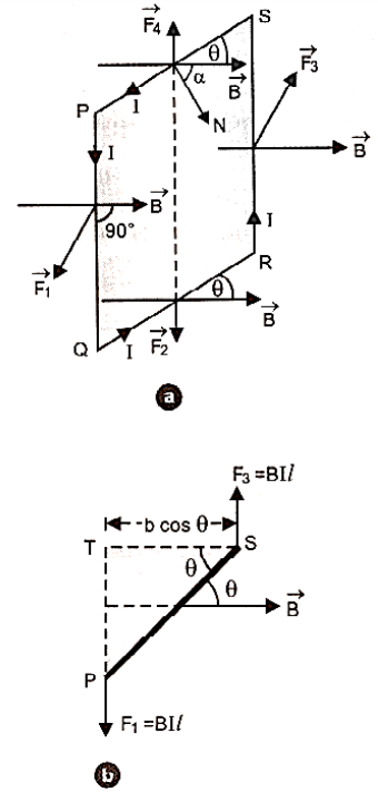
Let $\overrightarrow {{F_1}}$ ,$\overrightarrow {{F_2}} $, $\overrightarrow {{F_3}}$ \[\&\] $\overrightarrow {{F_4}} $ be the forces acting on the four current-carrying arms PQ, QR, RS and SP of the coil.
The force on arm SP is given by,
\[{\vec {F_4}} = {\text{I}}(\overrightarrow {{\text{SP}}} \times {\vec B}){\text{or}}{{\text{F}}_4} = {\text{I}}({\text{SP}}){\text{B}}\sin \left( {{{180}^ \circ } - \theta } \right) = {\text{IbB}}\sin \theta \]
The direction of this force is in the direction of $(\overrightarrow {SP} \times \overrightarrow {B)} $ i.e. in the plane of coil directed upwards.
The force on the arm QR is given by,
\[{\vec {F_2}} = {\text{I}}(\overrightarrow {{\text{QR}}} \times {\vec B})\] or \[{{\text{F}}_2} = {\text{I}}({\text{QR}}){\text{B}}\sin \theta = {\text{IbB}}\sin \theta \].
The direction of this force is in the plane of the coil directed downwards.
Because the forces $\overrightarrow {{F_2}} $ and $\overrightarrow {{F_4}} $ are of similar size and act in opposing directions along the same straight line, they cancel each other out, leaving the coil with no impact.
Now, the force on the arm PQ is given by,
\[{\vec {F_1}} = {\text{I}}(\overrightarrow {{\text{PQ}}} \times {\vec B}){\text{or}}{{\text{F}}_1} = {\text{I}}({\text{PQ}}){\text{B}}\sin {90^ \circ } = {\text{I}}\ell {\text{B}}(\because \overrightarrow {{\text{PQ}}} \bot {\vec B})\].
This force is projected outwards, perpendicular to the plane of the coil (i.e. perpendicular to the plane of paper directed towards the reader).
Force on the arm RS is given by,
\[{\vec {F_3}} = {\text{I}}(\overrightarrow {{\text{RS}}} \times {\vec B}){\text{or}}{{\text{F}}_3} = {\text{I}}({\text{PQ}}){\text{B}}\sin {90^ \circ } = {\text{I}}C{\text{B}}(\because \overrightarrow {{\text{RS}}} \bot {\vec B})\].
The direction of this force, is perpendicular to the plane of paper directed away from the reader i.e. into the plane of the coil.
The forces acting on the arms PQ and RS are equal, parallel, and acting in opposite directions with separate lines of action, forming a pair that causes the coil to revolve anticlockwise around the dotted line as axis.
The torque on the coil (equal to moment of couple) is given by:
\[\tau = {\text{either force}} \times {\text{arm of the couple}}\].
The forces F1 and F3 acting on the arms PQ and RS will be as shown in figure when seen from the top.
\[{{\text{Arm of couple}} = ST = PS\cos \theta = b\cos \theta } \]
\[{\tau = {\text{I}}\ell {\text{B}} \times {\text{b}}\cos \theta = {\text{IBA}}\cos \theta (\because \ell \times {\text{b}} = {\text{A}} = {\text{area of coil}}} \]
\[{{\text{PQRS}})}\]
If the rectangular coil has n turns, then
\[\tau = {\text{nIBA}}\cos \theta \]
Note that if the normal drawn on the plane of the coil makes an angle with the direction of magnetic field, then
\[\theta + \alpha = {90^ \circ }\]\[{\text{or}}\theta = {90^ \circ } - \alpha ;{\text{And}}\cos \theta = \cos \left( {{{90}^ \circ } - \alpha } \right) = \sin \alpha \].
Then the torque is given by,
\[\tau = {\text{nIBA}}\sin \alpha = {\text{MB}}\sin \alpha = |{\vec M}\times {\vec B}| = |{\text{nI\vec A}} \times {\vec B}|\] where \[{\text{nIA}} = {\text{M}}\]= magnitude of the magnetic dipole moment of the rectangular current loop.
\[\vec \tau = {\vec M} \times {\vec B} = {\text{nI}}({\vec A}\times {\vec B})\]
This torque tends to rotate the coil about its own axis. Its value changes with angle between plane of coil and direction of magnetic field.
Special Cases:
Case1:
If the coil is set with its plane parallel to the direction of magnetic field B, then \[\theta = {0^ \circ }{\text{and}}\cos \theta = 1\].
\[\therefore {\text{Torque,}}\tau = {\text{nIBA}}(1) = {\text{nIBA}}({\text{Maximum)}}\] .
This is the case with a radial field.
Case 2:
If the coil is set with its plane perpendicular to the direction of magnetic field B, then
\[\theta = {90^ \circ }{\text{and}}\cos \theta = 0\] . \[\therefore {\text{Torque,}}\tau = nIB{\text{A}}(0) = 0{\text{(Minimum)}}\].
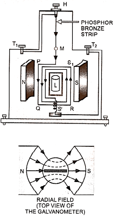
7. Moving Coil Galvanometer
A moving coil galvanometer is an instrument used for the detection and measurement of small electric currents.
Principle:
Its operation is based on the fact that a current-carrying coil encounters a torque when put in a magnetic field.
Construction:
It is made up of a coil PQRS1 with a large number of turns of insulated copper wire, as shown in the diagram. The coil is looped around a rectangular or circular non-magnetic metallic frame (typically brass). A phosphor bronze strip suspends the coil from a moveable torsion head H in a uniform magnetic field produced by two powerful cylindrical magnetic pole pieces N and S.
Moving Coil Galvanometer
The coil's bottom end is attached to one end of quartz or phosphor bronze hairspring S'. The terminal T2 is attached to the other end of this very elastic spring S'. If the coil is circular, the core is spherical; if the coil is rectangular, the core is cylindrical. It is held so tightly within the coil that it can freely rotate without hitting the iron core or pole parts. As a result, the magnetic field associated with the coil is a radial field. i.e. the coil's plane remains parallel to the magnetic field direction in all locations. The phosphor bronze strip has a concave mirror affixed to it. Using the lamp and scale arrangement, we can note the coil's deflection. To eliminate disruption from the air and other factors, the entire setup is housed in a nonmetallic container. At the base of the case, there are levelling screws.
For us, the spring S' performs three functions:
(i) It allows current to travel via the coil PQRS1.
(ii) It maintains the coil's position, and
(iii) it creates the twisted coil's restoring torque.
T1 is the terminal to which the torsion head is connected. Terminals T1 and T2 can be used to connect the galvanometer to the circuit.
Theory:
Suppose the coil PQRS1 is suspended freely in the magnetic field.
Let,
l = length PQ or RS1 of the coil,
b = breadth QR or S1 P of the coil,
n = number of turns in the coil.
Area of each turn of the coil, \[{\text{A}} = \ell \times {\text{b}}{\text{.}}\]
Let, B = strength of the magnetic field in which coil is suspended. I = current passing through the coil in the direction as shown in the figure.
Let be the angle formed by the normal drawn on the plane of the coil with the magnetic field direction at any given time.
As previously stated, when a rectangular coil carrying current is put in a magnetic field, it experiences a torque equal to \[\tau = {\text{nIBA}}\sin \alpha \].
If the magnetic field is radial i.e. the plane of the coil is parallel to the direction of the magnetic field then $\theta $=90° and \[ \sin \alpha\:=1\], \[\tau = {\text{nIBA}}\].
The coil rotates as a result of the torque. Twists occur in the phosphor bronze strip. As a result, a restoring torque is applied to the phosphor bronze strip, attempting to return the coil to its previous position. Let $\theta $ be the twist produced in the phosphor bronze strip due to rotation of the coil and k be the restoring torque per unit twist of the phosphor bronze strip, then total restoring torque produced k=$\theta $. In the equilibrium position of the coil, deflecting torque = restoring torque.
\[\therefore \quad {\text{nIBA}} = {\text{k}}\theta \]
\[I = \dfrac{{\text{k}}}{{{\text{nBA}}}}\theta {\text{orI}} = {\text{G}}\theta \]
Where \[\dfrac{{\text{k}}}{{{\text{nBA}}}} = {\text{G}} = {\text{a}}\]=constant for a galvanometer. It is known as galvanometer constant.
\[{\text{Hence,I}} \propto \theta \]
It means that the deflection caused by the galvanometer is proportionate to the current flowing through it. The scale on such a galvanometer is linear.
The deflection produced in a galvanometer when a unit current runs through it is defined as the current sensitivity of the galvanometer.
If \[\theta\] is the deflection in the galvanometer when current I is passed through it, then Current sensitivity,
\[{{\text{I}}_{\text{s}}} = \dfrac{\theta }{{\text{I}}} = \dfrac{{{\text{nBA}}}}{{\text{k}}}\quad \left( {\because {\text{I}} = \dfrac{{\text{k}}}{{{\text{nBA}}}}\theta } \right)\]
The unit of current sensitivity is $rad.{\text{ }}{A^{--1}}{\text{ }}or{\text{ }}div.{\text{ }}{A^{--1}}$
A galvanometer's voltage sensitivity is defined as the deflection produced when a unit voltage is applied across the two terminals of the galvanometer.
Let, V = voltage applied across the two terminals of the galvanometer,
$\theta $ = deflection produced in the galvanometer. Then, voltage sensitivity, ${v_s}$= $\theta $/V
If R = resistance of the galvanometer, I = current through it. Then V = IR
Voltage sensitivity, \[{{\text{V}}_{\text{S}}} = \dfrac{\theta }{{{\text{IR}}}} = \dfrac{{{\text{nBA}}}}{{{\text{kR}}}} = \dfrac{{{{\text{I}}_{\text{S}}}}}{{\text{R}}}\], \[{\text{the unit of}}{{\text{V}}_{\text{s}}}{\text{israd}}{{\text{V}}^{ - 1}}{\text{or div}}{\text{.}}{{\text{V}}^{ - 1}}{\text{.}}\]
Conditions for a Sensitive Galvanometer :
A galvanometer is said to be very sensitive if it shows large deflection even when a small current is passed through it, From the theory of galvanometer, \[\theta = \dfrac{{{\text{nBA}}}}{{\text{k}}}{\text{I}}\]. For a given value of I, will be large if $nBA/k$ is large. It is so if (a) n is large (b) B is large (c) A is large and (d) k is small
The value of n cannot be increased beyond a particular point since it causes the galvanometer's resistance to grow, as well as making the galvanometer bulky. This has the effect of lowering sensitivity. As a result, n cannot be increased indefinitely.
The value of B can be increased by using a strong horse shoe magnet.
Because the coil will not be in a uniform magnetic field if the value of A is increased beyond a certain point, the value of A cannot be increased beyond that point. Furthermore, it will make the galvanometer bulky and difficult to handle.
It is possible to reduce the value of k. The nature of the material used as a suspension strip determines the value of k. For quartz or phosphor bronze, the value of k is relatively low. As a result, a suspension strip made of quartz or phosphor bronze is utilised in sensitive galvanometers.
8. Ammeter
An ammeter is a low resistance galvanometer. It is used to measure the current in a circuit in amperes.
Using a low resistance wire in parallel with the galvanometer, a galvanometer can be transformed into an ammeter. The resistance of this wire (also known as the shunt wire) is determined by the ammeter's range can be computed as follows:
Let
G = Resistance of galvanometer,
n = Number of scale divisions in the galvanometer,
K = Figure of merit or current for one scale deflection in the galvanometer.
Then the current which produces full scale deflection in the galvanometer, \[{{\text{I}}_{\text{g}}} = {\text{nK}}\].
Let I be the maximum current be measured by a galvanometer.
\[I\overrightarrow {dl} {\text{ }} = {\text{ }}0 \]
To accomplish this, a shunt of resistance $S$ is connected in parallel with the galvanometer, with a portion of the total current ${I_g}$ flowing through the galvanometer and the remainder ($I - {I_g}$ ) flowing through the shunt figure.
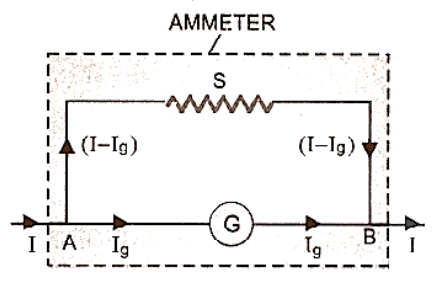
Circuit Diagram of Ammeter
\[{{\text{V}}_{\text{A}}} - {{\text{V}}_{\text{B}}} = {{\text{I}}_{\text{g}}}{\text{G}} = \left( {{\text{I}} - {{\text{I}}_{\text{g}}}} \right){\text{S}}\]
\[{\text{S}} = \left( {\dfrac{{{{\text{I}}_{\text{g}}}}}{{{\text{I}} - {{\text{I}}_{\text{g}}}}}} \right){\text{G}}\]
When this value of shunt resistance S is coupled in series with a galvanometer, it functions as an ammeter with a range of 0 to I ampere. The galvanometer's scale, which was recording the highest current I g before conversion to the ammeter, is now the same scale. When this value of shunt resistance S is coupled in series with a galvanometer, it functions as an ammeter with a range of 0 to I ampere. The same galvanometer scale that was recording the highest current I g before conversion into volts is now in use.
Note:
Initial reading of each division of the galvanometer to be used as ammeter is ${I_g}/n$ and the reading of the same each division after conversion into ammeter is $I/n$.
The effective resistance RP of ammeter (i.e. shunted galvanometer) will be
\[\dfrac{1}{{{{\text{R}}_{\text{P}}}}} = \dfrac{1}{{\text{G}}} + \dfrac{1}{{\text{S}}} = \dfrac{{{\text{S}} + {\text{G}}}}{{{\text{GS}}}}{\text{or}}{{\text{R}}_{\text{P}}} = \dfrac{{{\text{GS}}}}{{{\text{G}} + {\text{S}}}}\]
The combined resistance of the galvanometer and the shunt is very low since the shunt resistance is low, hence the ammeter has a significantly lower resistance than the galvanometer. The resistance of a perfect ammeter is zero.
9. Voltmeter
A voltmeter is a galvanometer with high resistance. It's a voltmeter that measures the potential difference between two locations in a circuit.
A galvanometer can be converted into a voltmeter by connecting a high resistance in series with the galvanometer. The value of the resistance depends upon the range of voltmeter and can be calculated as follows:
Let,
G = Resistance of galvanometer,
n = Number of scale divisions in the galvanometer,
K = Figure of merit of galvanometer i.e. current for one scale deflection of the galvanometer.
Current which produces full scale deflection in the galvanometer \[{{\text{I}}_{\text{g}}} = {\text{nK}}\]. Let V be the potential difference to be measured by the galvanometer. To accomplish so, a resistance R of this value is connected in series with the galvanometer, resulting in a current I g flowing through the galvanometer when a potential difference V is supplied between the terminals A and B figure.
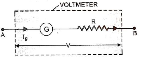
Now, total resistance of voltmeter = G + R
\[{\text{From Ohm's law,}}{{\text{I}}_{\text{g}}} = \dfrac{{\text{V}}}{{{\text{G}} + {\text{R}}}}{\text{orG}} + {\text{R}} = \dfrac{{\text{V}}}{{{{\text{I}}_{\text{g}}}}}\]
or
\[{\text{R}} = \dfrac{{\text{V}}}{{{{\text{I}}_{\text{g}}}}} - {\text{G}}\]
When this R value is linked in series with a galvanometer, it functions as a voltmeter with a range of 0 to V volts. Now, with two voltmeters, the same scale of the galvanometer that was recording the greatest potential I g G before conversion will record the potential V after conversion. It means that each division of the voltmeter's scale will indicate a higher potential than the galvanometer's. Effective resistance RS of converted galvanometer into voltmeter is:
\[{{\text{R}}_{\text{s}}} = {\text{G}} + {\text{R}}\]
Because a high resistance R is linked in series with the galvanometer in a voltmeter, the resistance of the voltmeter is much higher than that of the galvanometer. An ideal voltmeter's resistance is infinite.
10. Biotsavart’s Law
According to Biot-Savart’s law, the magnitude of the magnetic field induction dB (also called magnetic flux density) at a point P due to current element depends upon the factors at stated below :
${\text{dB}} \propto {\text{I}}$
\[{\text{dB}} \propto {\text{d}}\ell \]
\[{\text{dB}} \propto \sin \theta \]
\[{\text{dB}} \propto \dfrac{1}{{{{\text{r}}^2}}}\]
Combining these factors, we get:
\[ {{\text{dB}} \propto \dfrac{{{\text{Id}}\ell \sin \theta }}{{{{\text{r}}^2}}}}\]
\[{{\text{dB}} = {\text{K}}\dfrac{{{\text{Id}}\ell \sin \theta }}{{{{\text{r}}^2}}}}\] ……..(1)
where K is a constant of proportionality. Its value depends on the system of units chosen for the measurement of the various quantities and also on the medium between point P and the current element. When there is free space between current element and point, then:
In SI units,
\[{\text{K}} = \dfrac{{{\mu _0}}}{{4\pi }}{\text{and In cgs systemK}} = 1\] …….(2)
where ${\mu _o}$ is absolute magnetic permeability of free space.
\[{{\mu _0} = 4\pi \times {{10}^{ - 7}}{\text{Wb}}{{\text{A}}^{ - 1}}{{\text{m}}^{ - 1}} = 4\pi \times {{10}^{ - 7}}{\text{T}}{{\text{A}}^{ - 1}}{\text{m}}} \]
\[\left ({\because 1{\text{T}}} = 1 Wb\:{m^{-2}} \right ) \]
In SI units,
\[{\text{dB}} = \dfrac{{{\mu _0}}}{{4\pi }} \times \dfrac{{{\text{Id}}\ell \sin \theta }}{{{{\text{r}}^2}}}\] …(3)
In cgs system,
\[{\text{dB}} = \dfrac{{{\text{Id}}\ell \sin \theta }}{{{{\text{r}}^2}}}\]
In vector form, we may write:
\[|{\text{d{\vec B}}}| = \dfrac{{{\mu _0}}}{{4\pi }}\dfrac{{{\text{I}}|{\text{d}}\vec \ell \times {\vec r}|}}{{{{\text{r}}^3}}}{\text{ord\vec B}} = \dfrac{{{\mu _0}}}{{4\pi }}\dfrac{{{\text{I}}({\text{d}}\vec \ell \times {\vec r})}}{{{{\text{r}}^3}}}\] …(4)
The Direction of $\overrightarrow {dB} $:
From (4), the direction of dB must be the same as the direction of the cross product vector, d r. The right-handed screw rule, often known as the Right Hand Rule, is a representation of this. In this case, dB is perpendicular to the plane containing d and r and is pointing inwards. If the current element is to the left of the point P, dB will be perpendicular to the plane containing d and r and headed outwards.
Some Important Features of Biot Savart’s Law:
1. Biot Savart’s law is valid for a symmetrical current distribution.
2. Biot Savart’s law is applicable only to very small length conductor carrying current.
3. This law can not be easily verified experimentally as the current-carrying conductor of very small length can not be obtained practically.
4. This law is analogous to Coulomb’s law in electrostatics.
5. The direction of $\overrightarrow {dB} $ is perpendicular to both $I\overrightarrow {dl} $ and $\overrightarrow r $.
6. If \[\theta\:=\:{0^o}\] i.e. the point P lies on the axis of the linear conductor carrying current (or on the wire carrying current) then,
\[{\text{dB}} = \dfrac{{{\mu _0}}}{{4\pi }}\dfrac{{{\text{Id}}\ell \sin {0^ \circ }}}{{{{\text{r}}^2}}} = 0\].
That means there is no magnetic field induction at any point on the thin linear current-carrying conductor.
7. If \[\theta\:=\:{90^o}\] i.e. the point P lies at a perpendicular position w.r.t. current element, then
\[{\text{dB}} = \dfrac{{{\mu _0}}}{{4\pi }}\dfrac{{{\text{Id}}\ell }}{{{{\text{r}}^2}}}{\text{, which is maximum}}{\text{.}}\]
8. If \[\theta\:=\:{0^o}\] or \[180^o\], then
$d\overrightarrow B {\text{ }} = {\text{ }}0$i.e. minimum.
The magnetic field's Biot-law Savart's and the electrostatic field's Coulomb's law have similarities and differences.
Similarities:
Both the laws for fields are long range, since in both the laws, the field at a point varies inversely as the square of the distance from the source to point of observation.
Both the fields obey superposition principle.
The magnetic field is linear in the source $I\overrightarrow {dl} $ , just as the electric field is linear in its source, the electric charge q.
11. Magnetic Field Due to a Straight Conductor Carrying Current
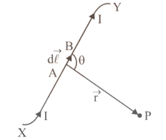
Figure 1 shows a straight wire conductor XY laying in the plane of paper carrying current I in the direction of X to Y. Let P be a point that is perpendicular to the straight wire conductor at a distance of a. PC clearly equals a. Allow small current elements to form the conductor.
Consider the straight wire conductor at O with a small current element $I\overrightarrow {dl} $. Let r be P's position vector relative to the current element, and be the angle between Id and r. Let's say CO = $l$.
Magnetic Field Due to a Current Carrying Conductor.
According to Biot-Savart’s law, the magnetic field $\overrightarrow {dB} $ (i.e. magnetic flux density or magnetic induction) at point P due to current element $I\overrightarrow {dl} $ is given by:
\[d{\vec B}=\dfrac {\mu_0}{4\pi}\dfrac {I\left ( \vec dl \times \vec r \right )}{r^3}\]
or \[{\text{dB}} = \dfrac{{{\mu _0}}}{{4\pi }} \times \dfrac{{{\text{Id}}\ell \sin \theta }}{{{{\text{r}}^2}}}\] …(5)
\[{\text{In rt}}{\text{. angled}}\vartriangle {\text{POC}},\theta + \phi = {90^ \circ }{\text{or}}\theta = {90^ \circ } - \phi \]
\[\therefore\:\sin \theta = \sin \left( {{{90}^ \circ } - \phi } \right) = \cos \phi \] …(6)
Also, \[\cos \phi = \dfrac{{\text{a}}}{{\text{r}}}{\text{or}}\quad {\text{r}} = \dfrac{{\text{a}}}{{\cos \phi }}\] …(7)
And, \[\tan \phi = \dfrac{\ell }{{\text{a}}}{\text{or}}\ell = {\text{a}}\tan \phi \]
On Differentiating it, we get:-
\[{\text{d}}\ell = {\text{a}}{\sec ^2}\phi {\text{d}}\phi \] …(8)
Putting the values in (5) from (6), (7) and (8), we get :
\[{\text{dB}} = \dfrac{{{\mu _0}}}{{4\pi }}\dfrac{{{\text{I}}\left( {{\text{ase}}{{\text{c}}^2}\phi {\text{d}}\phi } \right)\cos \phi }}{{\left( {\dfrac{{{{\text{a}}^2}}}{{{{\cos }^2}\phi }}} \right)}} = \dfrac{{{\mu _0}}}{{4\pi }}\dfrac{{\text{I}}}{{\text{a}}}\cos \phi {\text{d}}\phi \] …(9)
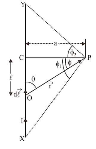
The direction of \[\overrightarrow {dB} \], according to right hand thumb rule, will be perpendicular to the plane of paper and directed inwards. As all the current elements of the conductor will also produce magnetic field in the same direction, therefore, the total magnetic field at point P due to current through the whole straight conductor XY can be obtained by integrating Eq. (9) within the limits – ${\phi _1} = {\phi _2} = {90^ \circ }$:
\[ = \dfrac{{{\mu _0}}}{{4\pi }}\dfrac{{\text{I}}}{{\text{a}}}\left[ {\sin {\phi _2} - \sin \left( { - {\phi _1}} \right)} \right] = \dfrac{{{\mu _0}}}{{4\pi }}\dfrac{{\text{I}}}{{\text{a}}}\left( {\sin {\phi _1} + \sin {\phi _2}} \right)\] …(10)
Special Cases:
When the conductor XY is of infinite length and the point P lies near the centre of the conductor then,
${\phi _1} = {\phi _2} = {90^ \circ }$
So, \[{\text{B}} = \dfrac{{{\mu _0}}}{{4\pi }}\dfrac{{\text{I}}}{{\text{a}}}\left[ {\sin {{90}^ \circ } + \sin {{90}^ \circ }} \right] = \dfrac{{{\mu _0}}}{{4\pi }}\dfrac{{2{\text{I}}}}{{\text{a}}}\]. …(11)
When the conductor XY is of infinite length but the point P lies near the end Y (or X) then,
\[{\phi _1} = {90^ \circ }{\text{and}}{\phi _2} = {0^ \circ }\]
\[{\text{B}} = \dfrac{{{\mu _0}}}{{4\pi }}\dfrac{{\text{I}}}{{\text{a}}}\left[ {\sin {{90}^ \circ } + \sin {0^ \circ }} \right] = \dfrac{{{\mu _0}}}{{4\pi }}\dfrac{{\text{I}}}{{\text{a}}}\] …(12)
The magnetic field due to an infinite long linear conductor carrying current near its centre is twice than that near one of its ends.
If length of conductor is finite, say L and point P lies on right bisector of conductor, then
\[{\phi _1} = {\phi _2} = \phi {\text{and}}\sin \phi = \dfrac{{{\text{L}}/2}}{{\sqrt {{{\text{a}}^2} + {{({\text{L}}/2)}^2}} }} = \dfrac{{\text{L}}}{{\sqrt {4{{\text{a}}^2} + {{\text{L}}^2}} }}\]
Then, \[{\text{B}} = \dfrac{{{\mu _0}{\text{I}}}}{{4\pi {\text{a}}}}[\sin \phi + \sin \phi ] = \dfrac{{{\mu _0}}}{{4\pi }}\dfrac{{2{\text{I}}}}{{\text{a}}}\sin \phi = \dfrac{{{\mu _0}}}{{4\pi }}\dfrac{{2{\text{I}}}}{{\text{a}}}\dfrac{{\text{L}}}{{\sqrt {4{{\text{a}}^2} + {{\text{L}}^2}} }}\]
When point P lies on the wire conductor, then \[{\text{d}}\vec \ell \]and \[{\vec r}\] for each element of the straight wire conductor are parallel. Therefore,\[{\text{d}}\vec \ell \times {\vec r} = 0\]. So the magnetic field induction at P = 0.
Direction of Magnetic Field:
Magnetic field lines caused by a current-carrying straight conductor take the shape of concentric circles with the conductor in the centre, lying in a plane perpendicular to the straight conductor. If current flows from A to B in a straight conductor, the direction of magnetic field lines is anticlockwise, and if current flows from B to A in a straight conductor, the direction is clockwise (b). Right Hand Thumb Rule or Maxwell's cork screw rule determines the direction of magnetic field lines.
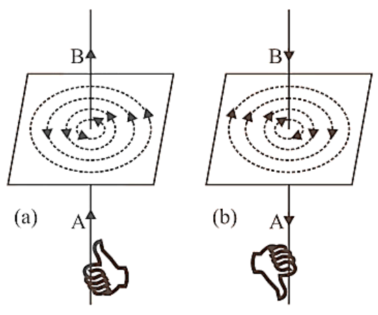
Direction of Magnetic Field
Right hand thumb rule. According to this rule, if we imagine the linear wire conductor to be held in the grip of the right hand so that the thumb points in the direction of current, then the curvature of the fingers around the conductor will represent the direction of magnetic field lines, figure (a) and (b).
Right Hand Thumb Rule
12. Magnetic Field at the Centre of the Circular Coil Carrying Current
Consider a circular coil with a radius of r and a centre of O that is lying in the plane of the paper. Assume I is the current flowing in the circular coil in the direction depicted in Figure. Assume the circular coil is made up of a huge number of current elements, each measuring dl in length.
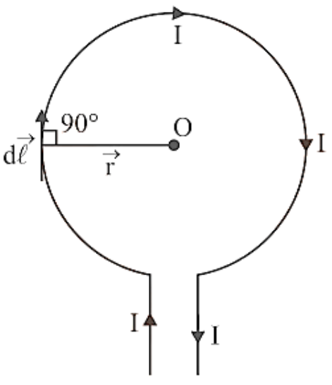
Magnetic Field in the Centre of the Circular Coil Carrying Current.
The magnetic field in the centre of the circular coil due to the current element Idl, according to Biot-Savart's law is given by
$d\vec B = \dfrac{{{\mu _0}}}{{4\pi }}I(\dfrac{{d\vec l \times \vec r}}{{{r^3}}})$ or $dB = \dfrac{{{\mu _0}}}{{4\pi }}\dfrac{{Id\vec lr\sin \theta }}{{{r^3}}} = \dfrac{{{\mu _0}}}{{4\pi }}\dfrac{{Idl\sin \theta }}{{{r^2}}}$
Where $\vec r$ is the position vector from point O. Now, the angle between \[d\vec l\] and $\vec r$ is 90°, therefore,
$dB = \dfrac{{{\mu _0}}}{{4\pi }}\dfrac{{Idl\sin {{90}^ \circ }}}{{{r^2}}}$ or $dB = \dfrac{{{\mu _0}}}{{4\pi }}\dfrac{{Idl}}{{{r^2}}}$ …(12)
The direction of dB in this situation is perpendicular to the plane of the current loop and inwards. Because current flowing through all parts of the circular coil contributes to the magnetic field in the same direction, the total magnetic field at point O due to current flowing through the entire circular coil may be calculated by integrating eq (12). Thus
$B = \int {dB = \int {\dfrac{{{\mu _0}}}{{4\pi }}} } \dfrac{{Idl}}{{{r^2}}} = \dfrac{{{\mu _0}}}{{4\pi }}\dfrac{I}{{{r^2}}}\int {dl} $
And we know,$\int {dl = } $total length of the circular coil = circumference of the current loop =$2\pi r$
$B = \dfrac{{{\mu _0}}}{{4\pi }}\dfrac{I}{{{r^2}}}.2\pi r = \dfrac{{{\mu _0}}}{{4\pi }}\dfrac{{2\pi l}}{r}$
Now if this coil consists of n number of loops, then
$B = \dfrac{{{\mu _0}}}{{4\pi }}\dfrac{{2\pi nI}}{r} = \dfrac{{{\mu _0}I}}{{4\pi r}} \times 2\pi n$ …(13)
i.e.\[B = \dfrac{{{\mu _0}I}}{{4\pi r}} \times \text{angle subtended by the coil at the center}.\]
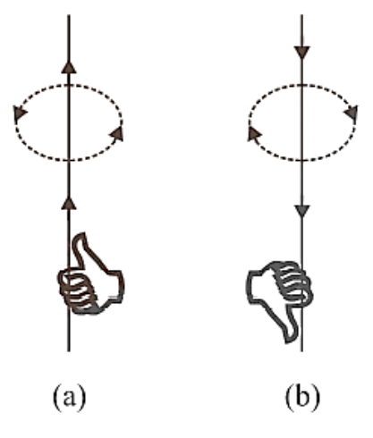
Direction of \[\vec B\]
Right hand rule determines the direction of the magnetic field at the centre of a circular current loop If we hold the thumb of the right hand perpendicular to the grip of the fingers in such a way that the curvature of the fingers represents the direction of current in the wire loop, the thumb of the right hand will point in the direction of magnetic field near the current loop's centre.
Direction of Magnetic Field Lines
13. Amperes’s Circuital Law
Consider a surface with a boundary C and current I flowing across it. Allow a huge number of small line elements, each with a length of dl, to make up the boundary C. The direction $d\vec l$ of the tiny line element under examination is tangential to its direction of dl. If ${B_t}$ is the tangential component of the magnetic field induction at this element, then ${B_t}$ and $d\vec l$ are both operating in the same direction, with no angle between them. For that element, we multiply ${B_t}$ by dl. Then
${B_t}dl = \vec B.d\vec l$
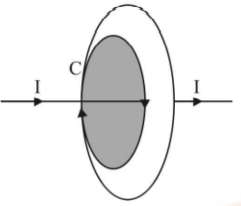
When the length dl is small and the products of all closed boundary components are summed together, the sum tends to be an integral around the closed route or loop (i.e.$\oint {} $,).
As a result, $\sum {} $of $\vec B.d\vec l$ over all items on a closed route = $\oint {\vec B.d\vec l} = $ B's line integral around the closed route or loop whose boundary corresponds with the closed path's border. Ampere's circuital law states that,
$\oint {\vec B.d\vec l = {\mu _0}} I$ …(19)
where I is the total current flowing through the closed route or loop and ${\mu _0}$ is the space's absolute permeability. Thus, the line integral of magnetic field induction $\vec B$ around a closed channel in vacuum equals ${\mu _0}$ times the total current I threading the closed path, according to Ampere's circuital equation.
The Right-Hand Rule specifies a sign convention for the sense of a closed path to be travelled while taking the line integral of the magnetic field (i.e., integration direction) and current threading it. According to it, if the curvature of the fingers of the right hand is perpendicular to the thumb of the right hand, and the curvature of the fingers represents the sense, the boundary is traversed in a closed path or loop for $\oint {\vec B.d\vec l} $, then the direction of the thumb gives the sense in which the current I is considered positive.
According to sign convention, ${I_1}$ is positive and ${I_2}$ is negative for the closed path depicted in figure. Then, according to Ampere's circuital Law, $\oint {\vec B.d\vec l = {\mu _0}({I_1} - {I_2}) = {\mu _0}{I_e}} $ where ${I_e}$ is the total current encompassed by the loop or closed route.
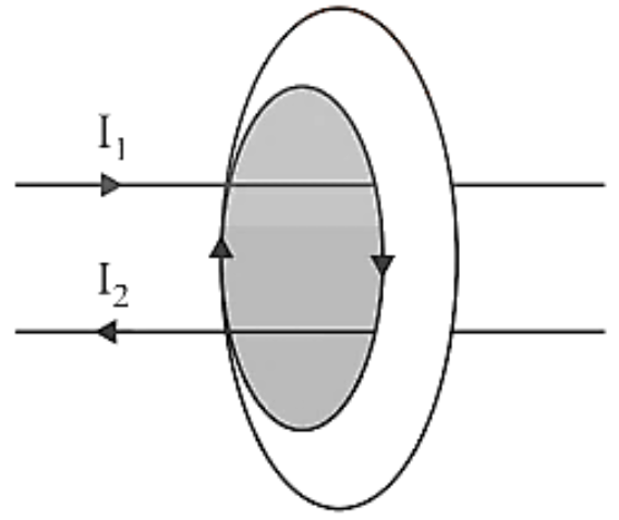
Diagram Depicting Current I1 is Positive and I2 is Negative for the Closed Path.
The size and geometry of the closed route or loop enclosing the current have no bearing on the relationship (19).
14. Magnetic Field Due to Infinte Long Wire Carrying Current
Consider an infinitely long straight line in a paper plane. Let I be the stream that flows from X to Y. A magnetic field is generated that has the same magnitude at all places at the same distance from the wire, i.e. the magnetic field is cylindrically symmetric around the wire.
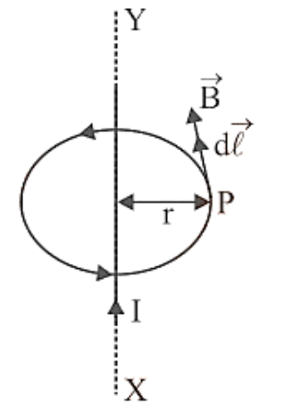
Magnetic Field Due To An Infinitely Long Current Carrying Wire.
Let P represent a location r away from the straight wire, and B represent the magnetic field at P. It will behave perpendicular to the magnetic field line that passes through P. Consider an amperian loop as a circle of radius r that is perpendicular to the plane of the paper and has its centre on wire, with point P lying on the loop, as shown in figure. At all places throughout this loop, the magnitude of the magnetic field is the same. The magnetic field B at P will be perpendicular to the circular loop's circumference. The amperian route will be integrated in an anticlockwise direction. Then B and d are both moving in the same direction. Around the closed loop, the line integral of B is
$\oint {\vec B.d\vec l = \oint {Bdl\cos {0^ \circ }} } = B\oint {dl = B2} \pi r$.
According to the sign convention, I is positive here.
Applying Ampere’s circuital law
$\oint {\vec B.d\vec l = {\mu _0}I} $ or $B2\pi r = {\mu _0}I$ or $B = \dfrac{{{\mu _0}I}}{{2\pi r}} = \dfrac{{{\mu _0}}}{{4\pi }}\dfrac{{2I}}{r}$ …(20)
15. Magnetic Field Due to Current Through a Very Long Circular Cylinder
Consider an infinitely long cylinder with axis XY and a radius R. Let's assume I current is flowing through the cylinder. Due to current flowing through the cylinder, a magnetic field is generated in the form of circular magnetic lines of force, the centres of which lie on the cylinder's axis. These force lines run parallel to the cylinder's length.
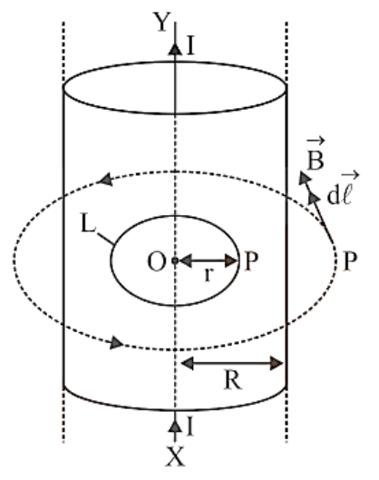
Case No. 1: Outside the cylinder is Point P. Let r be the perpendicular distance between point P and the cylinder axis, where r > R. Let $\vec B$ denote the induction of the magnetic field at P. It is acting in the direction of the magnetic line of force at P, which is directed into the paper. $\vec B$ and $d\vec l$ are acting in the same direction in this case.
Using the Ampere circuital rule, we've arrived at
\[{\oint {\mkern 1mu} \vec B \cdot d\vec \ell = {\mu _0}{\text{Ior}}\oint {\mkern 1mu} {\text{Bd}}\ell \cos {0^ \circ } = {\mu _0}{\text{I}}} \]
\[{{\text{or}}\,\,\oint {\mkern 1mu} {\text{Bd}}\ell = {\mu _0}{\text{Ior}}\,{\text{B}}2\pi {\text{r}} = {\mu _0}{\text{I}}} \]
Case No. 2: Here r < R. so have two possibilities.
If the current only flows along the cylinder's surface, as it does if the conductor is a cylindrical sheet of metal, current via the closed route L is zero. B = 0 is obtained using the Ampere circular law.
If the current is evenly distributed over the conductor's crosssection, the current through closed route L is given by
\[{\text{I'}} = \dfrac{{\text{I}}}{{\pi {{\text{R}}^2}}} \times \pi {{\text{r}}^2} = \dfrac{{{\text{I}}{{\text{r}}^2}}}{{{{\text{R}}^2}}}\]
Applying Ampere’s circuital law, we have
\[\oint {\mkern 1mu} {\mkern 1mu} {\vec B} \cdot {\text{d}}\vec \ell = {\mu _0}{\mu _{\text{r}}}{\text{I'}}\] or \[2\pi {\text{rB}} = {\mu _0}{\mu _{\text{r}}}{\text{I'}} = \dfrac{{{\mu _0}{\mu _{\text{r}}}{\text{I}}{{\text{r}}^2}}}{{{{\text{R}}^2}}}\] or \[{\text{B}} = \dfrac{{{\mu _0}{\mu _{\text{r}}}{\text{Ir}}}}{{2\pi {{\text{R}}^2}}}{\text{i}}{\text{.e}}{\text{.,B}} \propto {\text{r}}\]
For a current flowing through a solid cylinder, if we draw a graph between magnetic field induction B and distance from the axis of the cylinder, we get a curve of the type illustrated in figure.
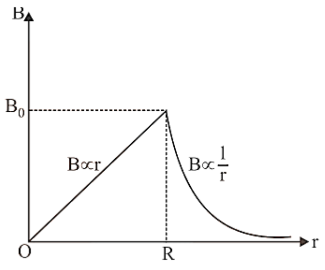
The magnetic field induction is greatest for a point on the surface of a solid cylinder carrying current and is zero for a point on the cylinder's axis.
16. Force Between Two Parllel Conducters Carrying Current
Consider two infinitely long straight conductors, ${C_1}{D_1}$ and ${C_2}{D_2}$, that carry currents \[{I_1}\] and ${I_2}$ in the same direction. In the plane of paper, they are kept parallel to each other at a distance of r. The magnetic field is created by current flowing through each conductor in the picture. Because each conductor is in the magnetic field created by the other, each conductor is subjected to a force.
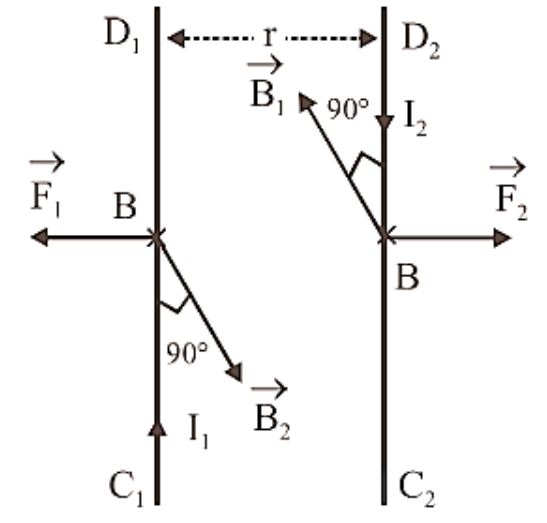
Due to current ${I_1}$ flowing through ${C_1}{D_1}$, magnetic field induction at a point P on conductor ${C_2}{D_2}$ is given by
\[{{\text{B}}_1} = \dfrac{{{\mu _0}}}{{4\pi }}\dfrac{{2{{\text{I}}_1}}}{{\text{r}}}\]. …(12)
The magnetic field ${B_1}$ is perpendicular to the plane of paper and directed inwards, according to the right hand rule. Because the current-carrying conductor ${C_2}{D_2}$ is located in the magnetic field ${B_1}$ (created by the current via ${C_1}{D_1}$), the unit length of ${C_2}{D_2}$ will be subjected to a force.
\[{{\text{F}}_2} = {{\text{B}}_1}{{\text{I}}_2} \times 1 = {{\text{B}}_1}{{\text{I}}_2}\]
Putting the value of ${B_1}$, we have
\[{{\text{F}}_2} = \dfrac{{{\mu _0}}}{{4\pi }} \cdot \dfrac{{2{{\text{I}}_1}{{\text{I}}_2}}}{{\text{r}}}\]
It indicates that two parallel linear conductors carrying currents in the same direction are attracted to one another.
One ampere is defined as the amount of current that, when flowing through two parallel uniform long linear conductors positioned one metre apart in free space, attracts or repels each other with a force of $2 \times {10^{ - 7}}N$ N per metre of their length.
17. The Solenoid
A solenoid is made out of an insulated long wire that is tightly wrapped into a helix shape. When compared to its diameter, it has a relatively long length.
Magnetic Field Due to a Solenoid
Consider a circular cross-sectioned long straight solenoid. Each of the solenoid's two turns is insulated from the other. When current is passed through the solenoid, each turn may be seen of as a current-carrying circular loop, and therefore a magnetic field is produced. The magnetic fields owing to neighbouring loops oppose each other at a location outside the solenoid, whereas the magnetic fields inside the solenoid are in the same direction. The effective magnetic field outside the solenoid weakens as a result, but the magnetic field within the solenoid becomes strong and homogeneous, operating along the solenoid's axis.
Let's use Ampere's circuital law now.
Let n be the number of turns per unit length of the solenoid, I be the current flowing through it, and the solenoid's turns be densely packed.
Figure 1 shows a rectangular amperian loop PQRS at the middle of the solenoid.
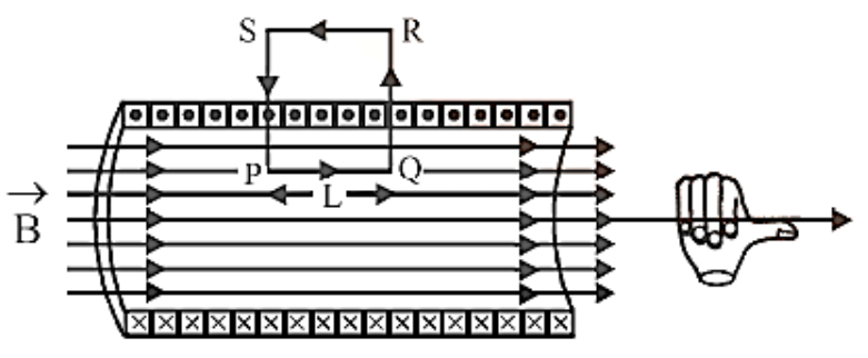
The line integral of magnetic field induction $\vec B$ over the closed path PQRS is:
\[\oint_{PQRS} \vec{B}\cdot \vec{dl}=\int_{P}^{Q}\vec{B}\cdot \vec{dl}+\int_{Q}^{R}\vec{B}\cdot \vec{dl}+\int_{R}^{S}\vec{B}\cdot \vec{dl}+\int_{S}^{P}\vec{B}\cdot \vec{dl}\]
Here,
\[\int_{P}^{Q}\vec{B}\cdot \vec{dl}=\int_{P}^{Q}Bdl\cos {0^o}=Bdl\]
and,
\[\int_{Q}^{R}\vec{B}\cdot \vec{dl}=\int_{Q}^{R}Bdl\cos {90^o}\:=\:0=\int_{S}^{P}\vec{B}\cdot \vec{dl}\]
Also,
$\int\limits_R^S {\vec B.d\vec l = 0} $ ($\because $outside the solenoid, B=0)
\[\oint {\mkern 1mu} {{\mkern 1mu} _{{\text{PQRS}}}}{\vec B} \cdot {\text{d}}\vec \ell = {\text{BL}} + 0 + 0 + 0 = {\text{BL}}\] …(1)
From Ampere’s circuital law
$\oint\limits_{PQRS} {\vec B.d\vec l = {\mu _0}} \times $total current through the rectangle PQRS
$ = {\mu _0} \times $no. turns in rectangle $ \times $current
$ = {\mu _0}nLI$ …(2)
From (1) and (2), we have
\[{\text{BL}} = {\mu _0}{\text{nLIorB}} = {\mu _0}{\text{nI}}\]
The magnetic field induction at a location well within the solenoid may be calculated using this equation. The magnetic field induction at a location near the end of a solenoid is determined to be ${\mu _0}n\dfrac{I}{2}$.
18. Toroid
The toroid is a hollow circular ring on which are tightly coiled a large number of insulated turns of a metallic wire. A toroid is, in reality, an infinite solenoid in the shape of a ring.
Toroid
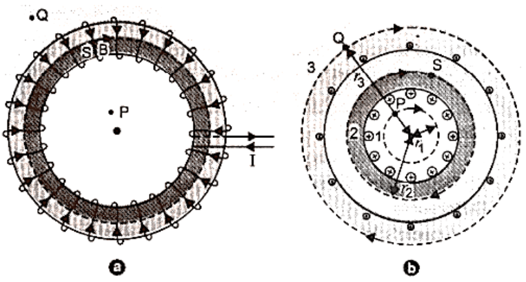
Magnetic Field Due to Current in an Ideal Toroid
Let I be the current flowing through the toroid and n be the number of rotations per unit length. The coil turns of an ideal toroid are round and tightly wrapped. Inside the toroid's turns, a magnetic field of constant magnitude is created in the form of concentric circular magnetic field lines. The tangent to the magnetic field line at a particular place determines the direction of the magnetic field there. We create three circular amperian loops of radii ${r_1}$, ${r_2}$, and ${r_3}$ to be traversed in a clockwise way, as shown in the figure by dashed circles, such that the points P, S, and Q might lie on them. The toroid is split in half by the circular region defined by loops 2 and 3. The loop 2 cuts each turn of current-carrying wire once, and the loop 3 cuts it twice. Let ${B_1}$ be the magnetic field magnitude along loop 1. Line integral of magnetic field ${B_1}$ along the loop 1 is
\[\oint {\mkern 1mu} {{\mkern 1mu} _{{\text{loop}}1}}{{\vec B}_1} \cdot {\text{d}}\vec \ell = \oint {\mkern 1mu} {{\mkern 1mu} _{{\text{loop}}1}}{{\text{B}}_1}{\text{d}}\ell \cos {0^ \circ } = {{\text{B}}_1}2\pi {{\text{r}}_1}\] …(i)
There is no current in Loop 1.
Ampere's circuital law states that
\[\oint {\mkern 1mu} {{\mkern 1mu} _{{\text{loop}}1}}{{\vec B}_1} \cdot {\text{d}}\vec \ell = {\mu _0} \times {\text{current enclosed by loop}}1 = {\mu _0} \times 0 = 0\]
\[{\text{or}}\quad {{\text{B}}_1}2\pi {{\text{r}}_1} = 0{\text{or}}{{\text{B}}_1} = 0\]
Let B3 be the magnetic field magnitude along loop 3.
The magnetic field B3's line integral along loop 3 equals
\[\oint {\mkern 1mu} {{\mkern 1mu} _{{\text{loop}}3}}{{\vec B}_3} \cdot {\text{d}}\vec \ell = \oint {\mkern 1mu} {{\mkern 1mu} _{{\text{loop}}3}}{{\text{B}}_3}{\text{d}}\ell \cos {0^ \circ } = {{\text{B}}_3}2\pi {{\text{r}}_3}\]
We can see from the sectional cut in figure that the current leaving the plane of paper is exactly negated by the current entering it. As a result, the total current contained within loop 3 is zero.
Ampere's circuital law states that
\[\oint\limits_{loop3} {{{\vec B}_3}.d\vec l} = {\mu _0} \times \text{total current through loop3} \]
\[or\,{B_3}2\pi {r_3} = {\mu _0} \times 0 = 0\,\,or\,{B_3} = 0 \]
Let B be the magnetic field magnitude along the loop. 2. The magnetic field line integral along loop 2 is
\[\oint {\mkern 1mu} {{\mkern 1mu} _{{\text{loop}}2}}{\vec B} \cdot {\text{d}}\vec \ell = {\text{B}}2\pi {{\text{r}}_2}\]
Current enclosed by the loop 2 = number of turns × current
in each turn =$2\pi {r_2}n \times I$
Ampere’s circuital law states that
\[\oint {\mkern 1mu} {{\mkern 1mu} _{{\text{loop}}2}}{\vec B} \cdot {\vec d}\vec \ell = {\mu _0} \times {\text{total current}}\]
or
\[B \left ( 2\pi{r_2} \right )=\mu_{0}\left ( 2\pi n{r_2}\ell \right )\]
\[B=\mu_{0}\;n\;\ell\]
19. Magnetism and Matter
The Bar Magnet
It's the most popular type of artificial magnet on the market. When we place a sheet of glass above a short bar magnet and sprinkle iron filings on it, the filings rearrange themselves as illustrated in figure. The pattern implies that attraction is greatest at the bar magnet's two ends. The magnet's poles are the opposite ends.
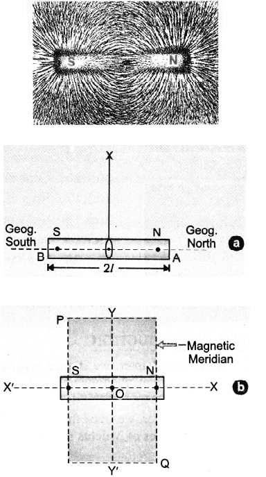
Magnetic Field Due To Bar Magnet
1. The earth has a magnetic field.
2. Each magnet attracts tiny particles of magnetic materials such as iron, cobalt, nickel, and steel.
3. When a magnet is held freely using an unspun thread, it comes to rest along the north-south axis.
4. Poles that are similar repel one other, whereas poles that are dissimilar attract each other.
5. The attraction or repulsion force F between two magnetic poles with strengths m1 and m2 separated by a distance r is proportional to the product of pole strengths and inversely proportional to the square of the distance between their centres, i.e.
\[{\text{F}} \propto \dfrac{{{{\text{m}}_1}{{\text{m}}_2}}}{{{{\text{r}}^2}}}{\text{orF}} = {\text{K}}\dfrac{{{{\text{m}}_1}{{\text{m}}_2}}}{{{{\text{r}}^2}}}\], where K is magnetic force constant.
In SI units, \[{\text{K}} = \dfrac{{{\mu _0}}}{{4\pi }} = {10^{ - 7}}{\text{Wb}}{{\text{A}}^{ - 1}}{{\text{m}}^{ - 1}}\]
where ${\mu _0}$is absolute magnetic permeability of free space (air/vacuum)
\[\therefore \quad {\text{F}} = \dfrac{{{\mu _0}}}{{4\pi }}\dfrac{{{{\text{m}}_1}{{\text{m}}_2}}}{{{{\text{r}}^2}}}\] … (1)
Coulomb's law of magnetic force describes this. K, on the other hand, has a value of 1 in the cgs system.
SI Unit of Magnetic Pole Strength
Suppose
\[{m_1} = {m_2} = m(say) \]
\[r = 1m\,and\,F = {10^{ - 7}}N \]
From equation (1),
\[{10^{ - 7}} = {10^{ - 7}} \times \dfrac{{({\text{m}})({\text{m}})}}{{{1^2}}}{\text{or}}{{\text{m}}^2} = 1{\text{orm}} = \pm 1\] ampere meter (Am).
When a magnetic pole repels an equal and comparable pole when put in vacuum (or air) at a distance of one metre from it with a force of ${10^{ - 7}}$ N, it is said to be one ampere-metre strong.
6. Magnetic poles are always found in pairs. Magnetic monopoles do not exist.
Direction of Magnetic Field at Point P
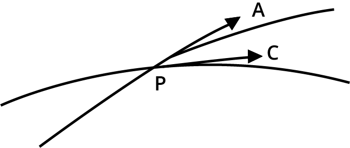
20. Magnetic Field Lines
The magnetic field line is an imaginary curve whose tangent at any point determines the direction of magnetic field B at that location. Imagine a magnet surrounded by a bunch of tiny compasses, due to the magnetic field, each compass needle is subjected to a torque. The torque operating on a compass needle aligns it with the magnetic field's direction.
The magnetic field line is the route along which the compass needles are oriented.
Properties of Magnetic Field Lines
1. A magnet's magnetic field lines (or the magnetic field lines of a current-carrying solenoid) create closed continuous loops.
2. Magnetic field lines extend from the north pole to the south pole outside the magnet's body.
3. The direction of the net magnetic field (B ) at any given place is represented by the tangent to the magnetic field line.
4. The number of magnetic field lines travelling properly through the unit area surrounding a place represents the amount of the magnetic field at that point. As a result, lines that are densely packed represent a high magnetic field, whereas lines that are sparsely packed represent a weak magnetic field.
5. There can be no crossing of magnetic field lines.
21. Magnetic Dipole
A magnetic dipole is made up of two poles that are diametrically opposed and separated by a short distance.
A bar magnet, a compass needle, and other magnetic dipoles are examples. A current loop will be shown to behave like a magnetic dipole. Due to electrons circling around the nucleus, an atom of a magnetic substance acts as a dipole.
The north pole and south pole of a magnetic dipole (or magnet) are always of equal intensity and are of opposing nature. Furthermore, such two magnetic poles always exist in pairs and cannot be separated.
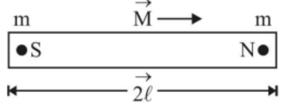
The magnetic length of a bar magnet is defined as the distance between its two poles. It is denoted by 2$\vec l$ and is a vector that runs from a magnet's S-pole to its N-pole.
The product of the strength of either pole (m) and the magnetic length (2$\vec l$ ) of the magnet is the magnetic dipole moment.
$\vec M$ is the symbol for it.
The magnetic dipole moment is equal to the strength of either pole multiplied by the magnetic length.
\[{\vec M} = {\text{m}}(2\vec \ell )\]
The magnetic dipole moment is a vector quantity that runs from the magnet's south pole to its north pole, as shown in figure.
We shall show that the SI unit of M is joule/tesla or ampere Metre2
$\therefore $SI unit of pole strength is Am.
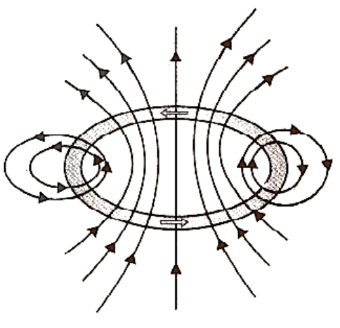
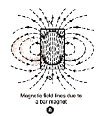
Bar Magnet as an Equivalent Solenoid
A current loop is known to function as a magnetic dipole.
All magnetic phenomena, according to Ampere's idea, may be described in terms of circulating currents. Magnetic field lines for a bar magnet and a current-carrying solenoid are quite similar in figure. As a result, a bar magnet, like a solenoid, may be conceived of as a huge number of circulating currents. A bar magnet is similar to a solenoid in that it may be cut. Two smaller solenoids with lesser magnetic characteristics are delivered. The magnetic field lines stay continuous, coming from one solenoid's face and entering the second solenoid's face. If we move a tiny compass needle between a bar magnet and a current-carrying solenoid, we will see that the deflections of the needle are identical in both situations.
Calculate the axial field of a finite solenoid carrying the current to illustrate the resemblance of a current-carrying solenoid to a bar magnet.
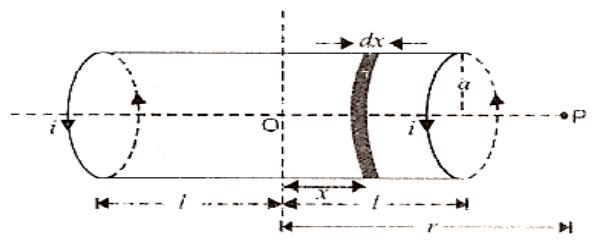
Assume a = solenoid radius and 2 = solenoid length with the centre in the diagram. O
n is the number of turns per unit length of the solenoid, and I is the current intensity that passes through it.
We must determine the magnetic field at any point P on the solenoid's axis, where OP = r. Consider a tiny solenoid element with a thickness of dx and a distance of x from O.
The element's number of turns is equal to n dx.
The magnitude of the magnetic field at P owing to this current element may be calculated using equation.
\[{\text{dB}} = \dfrac{{{\mu _0}{\text{i}}{{\text{a}}^2}({\text{ndx}})}}{{2{{\left[ {{{({\text{r}} - {\text{x}})}^2} + {{\text{a}}^2}} \right]}^{3/2}}}}\]
If P lies at a very large distance from O, i.e., r >> a and r >> x, then
\[{\left[ {{{({\text{r}} - {\text{x}})}^2} + {{\text{a}}^2}} \right]^{3/2}} \approx {{\text{r}}^3}\]
\[{\text{dB}} = \dfrac{{{\mu _0}{\text{i}}{{\text{a}}^2}{\text{ndx}}}}{{2{{\text{r}}^3}}}\] …(1)
Because the range of x is from x = – l to x = +l, the amplitude of the total magnetic field at P owing to the current-carrying solenoid is also from x = – l to x = +l .…(2)
If M is the solenoid's magnetic moment, then M = total number of turns x current x cross section area
\[{\text{M}} = {\text{n}}(2\ell ) \times {\text{i}} \times \left( {\pi {{\text{a}}^2}} \right)\]
\[\therefore \quad {\text{B}} = \dfrac{{{\mu _0}}}{{4\pi }}\dfrac{{2{\text{M}}}}{{{{\text{r}}^3}}}\] …(3)
The magnetic field on the axial line of a short bar magnet is expressed in this way.
As a result, the axial field of a current-carrying finite solenoid is identical to that of a bar magnet. As a result, a finite solenoid carrying current is functionally equal to a bar magnet.
Potential Energy of a Magnetic Dipole in a Magnetic Field
A magnetic dipole's potential energy in a magnetic field is the energy that the dipole has owing to its specific location in the field.
The magnitude of the torque operating on a magnetic dipole of moment $\vec M$ is when it is maintained at an angle with the direction of a uniform magnetic field B.
\[\tau = {\text{MB}}\sin \theta \] …(1)
This torque causes the dipole to align in the field's direction. Work must be done to rotate the dipole against the torque's action. This work is stored as dipole potential energy in the magnetic dipole.
Now, the dipole is rotated via a tiny angle d against the restoring torque with a modest amount of effort.
\[{\text{dW}} = \tau {\text{d}}\theta = {\text{MB}}\sin \theta {\text{d}}\theta \]
Total work done in rotating the dipole from $\theta = {\theta _1}\,to\,\theta = {\theta _2}$is
$\therefore $ Potential energy of the dipole is
\[{\text{U}} = {\text{W}} = - MB\left( {\cos {\theta _2} - \cos {\theta _1}} \right)\] …(2)
When \[{\theta _1} = {90^ \circ },\,and\,{\theta _2} = \theta \],then
\[{\text{U}} = {\text{W}} = - {\text{MB}}\left( {\cos \theta - \cos {{90}^ \circ }} \right)\]
\[{\text{W}} = - {\text{MB}}\cos \theta \] …(3)
In vector notation, we may rewrite (3) as
\[{\text{U}} = - {\vec M} \cdot {\vec B}\] …(4)
Particular Cases
1. When $\theta = {90^ \circ }$
\[{\text{U}} = - {\text{MB}}\cos \theta = - {\text{MB}}\cos {90^ \circ } = 0\]
The dipole's potential energy is 0 when it is perpendicular to the magnetic field.
As a result, to compute the potential energy of a dipole at any angle with B, we utilise
\[{\text{U}} = - {\text{MB}}\left( {\cos {\theta _2} - \cos {\theta _1}} \right)\] and take ${\theta _1} = {90^ \circ }\,and\,{\theta _2}\, = \,\theta .$
Therefore,
\[{\text{U}} = - {\text{MB}}\cos {0^ \circ } = - {\text{MB}}\]
2. When $\theta = {0^ \circ }$
\[{\text{U}} = - {\text{MB}}\cos {0^ \circ } = - {\text{MB}}\]
it is the bare minimum. This is the point of stable equilibrium, which occurs when the magnetic dipole is oriented along the magnetic field and has the lowest P.E.
3. When $\theta = {180^ \circ }$
\[{\text{U}} = - {\text{MB}}\cos {180^ \circ } = {\text{MB}}\]which is maximum. This is the position of unstable equilibrium.
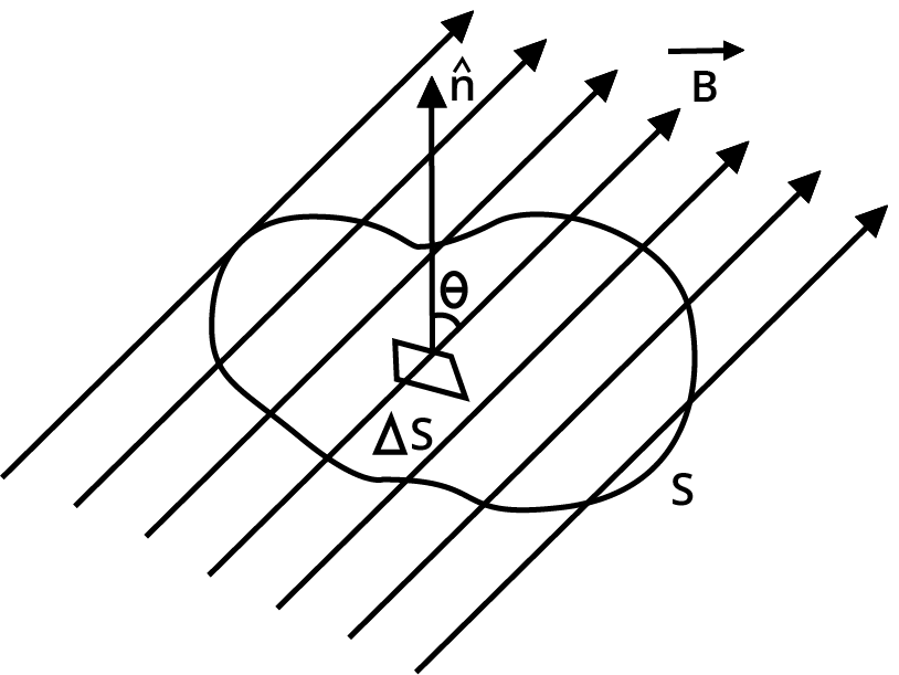
Diagram Showing the Angle Between Magnetic Field And Surface Normal.
22. Magnetism and Gauss Law
The net magnetic flux (B ) through any closed surface is always zero, according to Gauss's law of magnetism.
23. Earth’s Magnetism
Magnetic Declination
The angle between the magnetic meridian and the geographic meridian at a given location is known as magnetic declination.
Magnetic Declination
Retain in Memory
1. The magnetic poles of the planet are not exactly opposite each other on the globe. Magnetic south is currently further away from geographic south than magnetic north is from geographical north.
2. In truth, the earth's magnetic field fluctuates with both place and time. For example, the magnetic declination in London changed by 3.5° over a 240-year period from 1580 to 1820 A.D., implying that the earth's magnetic poles shift position over time.
3. India's magnetic declination is rather modest. The declination at Delhi is just 0° 41' East, but at Mumbai it is 0° 58' West. The compass needle properly indicates the direction of geographic north in each of these locations (within 1° of the true direction).
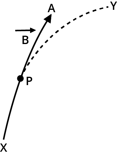
Magnetic Dip or Magnetic Inclination
The angle formed by the direction of overall intensity of the earth's magnetic field and a horizontal line in the magnetic meridian is known as magnetic dip or magnetic inclination.
Horizontal Component
It is the horizontal component of the overall strength of the earth's magnetic field in the magnetic meridian. H. is the one who represents it.
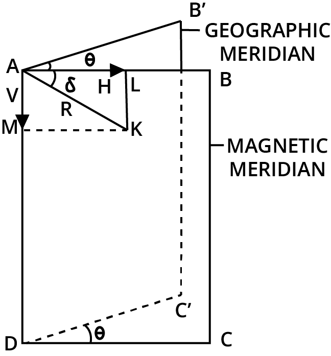
The entire intensity of the earth's magnetic field is represented by AK in the diagram,\[\angle {\text{BAK}} = \delta \] .
The resulting intensity R along AK is broken down into two rectangles:
Along AB, the horizontal component is:
\[{\text{AL}} = {\text{H}} = {\text{R}}\cos \delta \] …(1)
Vertical component along AB is
\[{\text{AM}} = {\text{V}} = {\text{R}}\sin \delta \]. …(2)
(1) and (2) are squared, and they are added.
\[{{\text{H}}^2} + {{\text{V}}^2} = {{\text{R}}^2}\left( {{{\cos }^2}\delta + {{\sin }^2}\delta } \right) = {{\text{R}}^2}\].
$\therefore R = \sqrt {{H^2} + {V^2}} $ …(3)
Dividing (1) by (2), we get
\[\dfrac{{{\text{R}}\sin }}{{{\text{R}}\cos }} = \dfrac{{\text{V}}}{{\text{H}}}{\text{or}}\quad \tan = \dfrac{{\text{V}}}{{\text{H}}}\] …(4)
The value of the horizontal component \[{\text{H}} = {\text{R}}\cos \delta \] varies depending on where you look. $\delta = {90^ \circ }$ at the magnetic poles
\[\therefore \quad {\text{H}} = {\text{R}}\cos {90^ \circ } = {\text{zero}}\]
At the magnetic equator, $\delta = {0^ \circ }$
\[\therefore \quad {\text{H}} = {\text{R}}\cos {0^ \circ } = {\text{R}}\]
Both a vibration magnetometer and a deflection magnetometer can be used to measure the horizontal component (H).
The value of H at a given location on the earth's surface is on the order of 3.2 10–5 tesla.
Memory Note
Above the surface of the earth, the horizontal component H of the magnetic field runs from geographic south to geographic north. (if declination is ignored)
24. Magnetic Properties of Matter
We define the following words to explain the magnetic characteristics of materials, which should be understood well.
Magnetic Permeability
The capacity of a material to allow the passage of magnetic lines of force through it, i.e. the degree or extent to which a magnetic field may penetrate or permeate it, is referred to as relative magnetic permeability. It's symbolised as ${\mu _r}$
The ratio of the number of magnetic field lines per unit area (i.e. flux density B) in a material to the number of magnetic field lines per unit area that would be present if the medium were replaced by vacuum is known as relative magnetic permeability. (i.e. ${B_0}$ flux density)
\[{\mu _{\text{r}}} = \dfrac{{\text{B}}}{{{{\text{B}}_0}}}\]
The ratio of magnetic permeability of the material ($\mu $) to magnetic permeability of empty space (\[{\mu _0}\]) may also be used to determine relative magnetic permeability of a material.
\[\therefore \quad {\mu _{\text{r}}} = \dfrac{\mu }{{{\mu _0}}}{\text{or}}\quad \mu = {\mu _{\text{r}}}{\mu _0}\]
We know that \[{\mu _0} = 4\pi \times {10^{ - 7}}{\text{weber/amp - metre}}\left( {{\text{Wb}}{{\text{A}}^{ - 1}}{{\text{m}}^{ - 1}}} \right)\]
$\therefore $ SI units of permeability are \[{\text{H}}{{\text{m}}^{ - 1}} = {\text{Wb}}{{\text{A}}^{ - 1}}{{\text{m}}^{ - 1}} = \left( {{\text{T}}{{\text{m}}^2}} \right){{\text{A}}^{ - 1}}{{\text{m}}^{ - 1}} = {\text{Tm}}{{\text{A}}^{ - 1}}\]
\[{\text{H}}{{\text{m}}^{ - 1}} = {\text{Wb}}{{\text{A}}^{ - 1}}{{\text{m}}^{ - 1}} = \left( {{\text{T}}{{\text{m}}^2}} \right){{\text{A}}^{ - 1}}{{\text{m}}^{ - 1}} = {\text{Tm}}{{\text{A}}^{ - 1}}\].Magnetic Intensity ($\vec H$)
The magnetising force or magnetise intensity ($\vec H$) of a magnetic field is a measure of its ability to magnetise a substance.
Magnetisation or Intensity of Magnetisation ‘I’
When a specimen is placed in a magnetising field, it shows how much it is magnetised. A magnetic substance's magnetisation is described quantitatively as the magnetic moment per unit volume of the material.
\[({\text{M}}) = \dfrac{{{\text{Magnetic moment}}}}{{{\text{volume}}}} = \dfrac{{\text{m}}}{{\text{V}}}\]
There are SI units for I that are identical to SI units for H.
The ratio of the intensity of magnetisation (I) generated in the material to the magnetising force (H) put on it is described as magnetic susceptibility (${\chi _m}$) of a magnetic material. Magnetic susceptibility is denoted by${\chi _m}$.
Thus ${\chi _m} = \dfrac{I}{H}$
Relation Between Magnetic Permeability and Magnetic Susceptibility
A magnetic substance becomes magnetised when it is put in a magnetising field of magnetising strength H. The total magnetic induction B in the material is equal to the sum of the magnetic induction ${B_0}$ in vacuum caused by the magnetic intensity and the magnetic induction ${B_m}$ caused by the material's magnetisation.
Therefore,
$B = {B_0} + {B_m}$
But ${B_0} = {\mu _0}H$ and ${B_m} = {m_0}I$,where I is the magnetic material's induced magnetisation intensity. As a result of the foregoing,
\[{\text{B}} = {\mu _0}{\text{H}} + {\mu _0}{\text{I}} = {\mu _0}({\text{H}} + {\text{I}})\]
i.e. \[{\text{B}} = {\mu _0}({\text{H}} + {\text{I}})\]
Now as \[{\chi _{\text{m}}} = \dfrac{{\text{I}}}{{\text{H}}}\quad \therefore {\text{I}} = {\chi _{\text{m}}}{\text{H}}\]
From above, \[{\text{B}} = {\mu _0}\left( {{\text{H}} + {\chi _{\text{m}}}{\text{H}}} \right) = {\mu _0}{\text{H}}\left( {1 + {\chi _{\text{m}}}} \right)\]
But $B = \mu H$
\[\therefore \quad \mu {\text{H}} = {\mu _0}{\text{H}}\left( {1 + {\chi _{\text{m}}}} \right){\text{or}}\dfrac{\mu }{{{\mu _0}}} = 1 + {\chi _{\text{m}}}\]
or \[{\mu _{\text{r}}} = 1 + {\chi _{\text{m}}}\]
This is the relationship between the material's magnetic susceptibility and its relative magnetic permeability.
25. Classification of Magnetic Materials
On Earth, there are many different elements and compounds.
In the laboratory, new elements, alloys, and compounds have been created. These compounds were categorised by Faraday into three groups based on their magnetic properties:
(i) Diamagnetic materials, (ii) Paramagnetic materials, and (iii) Ferromagnetic materials
Their main characteristics are discussed below :
Diamagnetic Substances
Individual atoms/molecules/ions in diamagnetic substances have no net magnetic moment on their own. When such substances are exposed to an external magnetising field, they become weakly magnetised in the opposite direction.
These compounds have a tendency to migrate from stronger regions of the magnetic field to weaker sections when exposed to a non-uniform magnetic field.
When a diamagnetic material specimen is placed in a magnetising field, the magnetic field lines choose not to pass through it.
The relative magnetic permeability of diamagnetic materials is never more than one.
From the relation\[{\mu _{\text{r}}} = \left( {1 + {\chi _{\text{m}}}} \right),{\text{a}}{\mu _{\text{r}}} < 1,{\chi _{\text{m}}}\] is negative
As a result, diamagnetic susceptibility has a tiny negative value.
A magnet repels a superconductor, and the magnet repels the superconductor.
The Meissner effect refers to the occurrence of complete diamagnetism in superconductors. Magnetically levitated speedy trains have been run using superconducting magnets.
Paramagnetic Substances
Paramagnetic substances are those in which each atom, molecule, or ion has its own net non-zero magnetic moment. When such materials are exposed to an external magnetic field, they become weakly magnetised in the direction of the field.
They tend to migrate from weaker areas of the field to stronger sections when placed in a non-uniform magnetic field.
When a paramagnetic material specimen is placed in a magnetising field, the magnetic field lines prefer to travel through the specimen rather than through the air.
From the SI relation,\[{\mu _{\text{r}}} = 1 + {\chi _{\text{m}}},{\text{as}}{\mu _{\text{r}}} > 1\], therefore, ${\chi _m}$must be positive.
As a result, the susceptibility of paramagnetic materials is positive, albeit modest.
The susceptibility of paramagnetic substances changes inversely with their temperature, i.e. ${\chi _m} \propto \dfrac{1}{T}$, i.e. they lose their magnetic property as the temperature rises.
Ferromagnetic Substances
In contrast to paramagnetic substances, ferromagnetic substances have a non-zero magnetic moment for each individual atom, molecule, or ion.
When such materials are exposed to an external magnetic field, they become highly magnetised in the field's direction.
All of the characteristics of paramagnetic materials are present in ferromagnetic materials, but to a considerably higher extent. For example
I They are highly magnetised in the direction of the external field they are in.
(ii) Ferromagnetic materials have a very high relative magnetic permeability $( \approx {10^{3\,}}\,to\,{10^5})$
(iii) Ferromagnetic materials have a very high susceptibility$(\because {\chi _m} = {\mu _r} - 1)$
As a result, they are easily and powerfully magnetised.
(iv) Ferromagnetic susceptibility diminishes as temperature rises. The transition from ferromagnetics to paramagnetics occurs at a particular temperature. The temperature at which this transition occurs is known as the curie temperature. Curie temperature of iron, for example, is around 1000 K.
Curie Law in Magnetism
The intensity of magnetisation (I) of a magnetic material is I directly proportional to magnetic induction (B) and (ii) inversely proportional to the material's temperature (T) according to Curie's law,i.e. \[I \propto B,\]and $I \propto \dfrac{1}{T}$
Combining these factors we get $I \propto \dfrac{B}{T}$
As $B \propto H$, magnetising intensity
\[\therefore \quad {\text{I}} \propto \dfrac{B}{{\text{T}}}{\text{orI}} \propto \dfrac{1}{{\text{T}}}\]
But $\dfrac{I}{H} = {\chi _m}$
\[\therefore \quad {\chi _{\text{m}}} \propto \dfrac{1}{{\text{T}}}{\text{or}}\quad {\chi _{\text{m}}} = \dfrac{{\text{C}}}{{\text{T}}}\]
C stands for the Curie constant, which is a proportionality constant.
26. Hysteresis Curve
The hysteresis curve depicts the relationship between a ferromagnetic material's magnetic induction $\vec B$ (or intensity of magnetization $\vec I$ ) and the magnetising force or magnetic intensity $\vec H$. The hysteresis curve's form is seen in figure. It depicts the behaviour of the material as it goes through a magnetization cycle.
Assume that the material is initially unmagnetized, i.e. $\vec B = 0$ and H$\vec H = 0$. The origin O is used to denote this condition. We put the material in a solenoid and progressively raise the current through it. $\vec H$ enhances the magnetising force. As seen in the curve oa, the magnetic induction $\vec B$in the material rises and saturates. This behaviour indicates that the domains of ferromagnetic material are aligning and merging until no more $\vec B$ enhancement is feasible. As a result, increasing solenoid current and hence magnetic strength beyond this point is pointless.
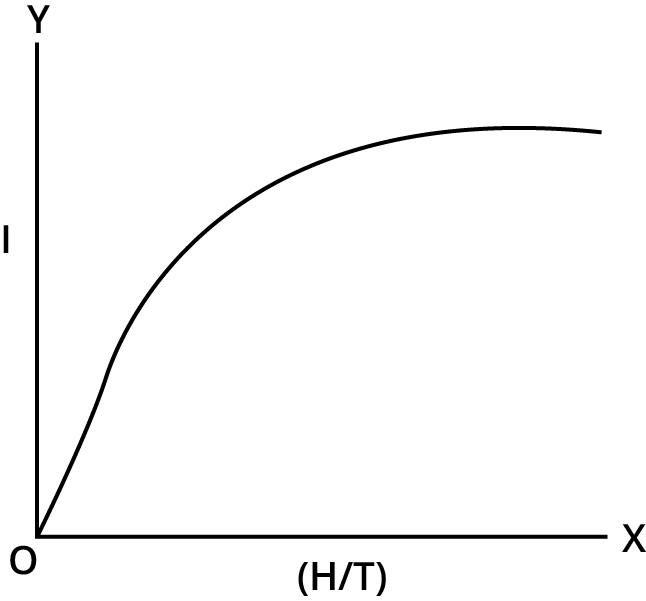
Graph Between Intensity Of Magnetization and H/T
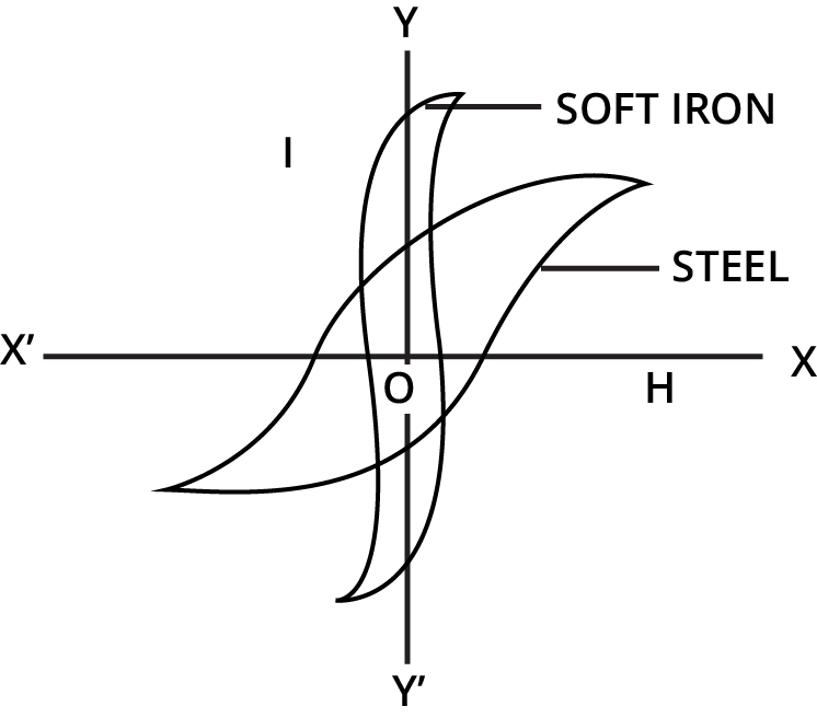
Hysteresis Curve
The solenoid current, and therefore magnetic strength $\vec H$ is then reduced until it reaches zero. The curve follows the route ab, indicating that when $\vec H = 0,\,\vec B \ne 0.$. As a result, some magnetism remains in the specimen.
When the magnetising force is decreased to zero, the value of magnetic induction $\vec B$ remaining in the specimen is called Retentivity, Remanence, or Residual magnetism of the material.
Even after the magnetising force is eliminated, the domains are not entirely randomised. The current in the solenoid is then reversed and gradually raised.
The net magnetic induction B within is lowered to zero by flipping some domains. The curve bc is a representation of this. To reduce residual magnetism or retentivity to zero, a magnetising force = OC in the opposite direction must be applied. The coercivity of a substance is the value of its magnetising force.
We get saturation in the reverse direction at d as the amplitude of the reverse current in the solenoid increases. The curve cd is used to depict variation. The solenoid current is then decreased (curve de), reversed, and raised (curve ea). The cycle continues to repeat itself. The saturated magnetic induction BS is of the order of 1.5 T, and the coercivity is on the order of $ - 90A{m^{ - 1}}$.
It is evident from the preceding explanation that when a magnetic material specimen is subjected to a cycle of magnetisation, the intensity of magnetisation (I) and magnetic induction (B) lag behind the magnetising force (H). As a result, even if the magnetising force H is reduced to zero, the values of I and B do not decrease to zero, indicating that the specimen retains its magnetic characteristics.
Hysteresis is the occurrence of I or B trailing behind H when a magnetic material specimen is exposed to a cycle of magnetisation.
The hysteresis loop for soft iron, for example, is narrow and big, whereas the hysteresis loop for steel is wide and short, as seen in figure.
Hysteresis Curve for Soft Iron and Steel
The hysteresis loops of soft iron and steel indicate that
(isoft iron's retentivity is larger than steel's retentivity,
soft iron is more strongly magnetised than steel, and
soft iron's coercivity is lower than steel's coercivity. It indicates that soft iron loses its magnetic faster than steel.
hysteresis loss in soft iron is less than hysteresis loss in steel because the area of the I-H loop for soft iron is smaller than the size of the I-H loop for steel.
Permanent Magnets
Permanent magnets are materials that keep their ferromagnetic characteristics for a long period at room temperature.
The selected material should have
A high retentivity so that the magnet is strong, and
A high coercivity so that the magnetisation is not erased by stray magnetic fields, temperature changes, or mechanical damage due to rough handling, among other things.
High permeability, allowing for easy magnetisation.
Permanent magnets are often made of steel.
Electromagnets
Electromagnets have ferromagnetic materials at their core, which have a high permeability and low retentivity.
Soft iron is a good choice for this project. When a soft iron rod is inserted into a solenoid and a current is sent through it, the solenoid's magnetic is multiplied by a thousand. Because the retentivity of soft iron is relatively low, when the solenoid current is turned off, the magnetism is immediately eliminated. Electric bells, loudspeakers, and telephone diaphragms all employ electromagnets. Cranes utilise massive electromagnets to raise machines and other items.
Magnetic field at centre O in Different Conditions of Circular Current.
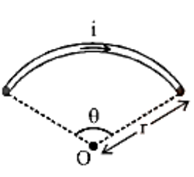
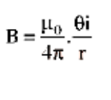
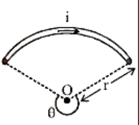
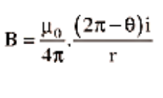
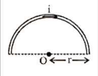
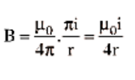
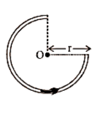
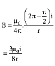
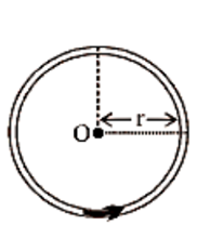
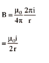
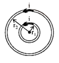
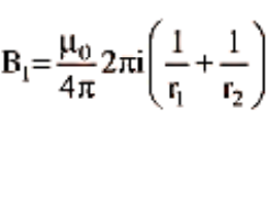
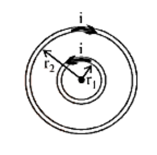

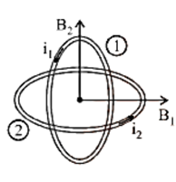

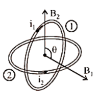

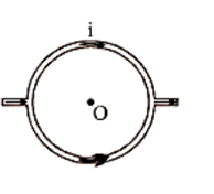

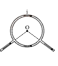

27. Hall Effect
The Hall effect is the phenomenon of creating a transverse emf in a current-carrying conductor by introducing a magnetic field perpendicular to the current direction.
We may use the Hall effect to determine the kind and quantity of charge carriers in a conductor.
Consider a conductor with current carriers that are electrons.
The electrons travel with a drift velocity of v in the opposite direction of current flow.
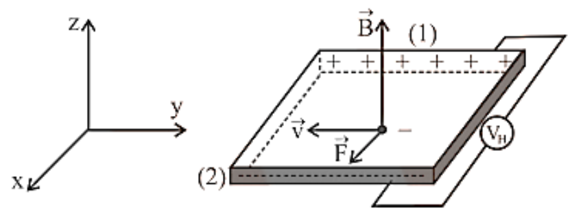
Force acting on electron \[{{\text{F}}_{\text{m}}} = - {\text{e}}({\vec v} \times {\vec B})\].This force works along the x-axis, causing electrons to migrate towards face (2), making it negatively charged.
28. Standard Cases for Force on Current-Carrying Conductors
Case 1:
When an arbitrary current-carrying loop is put in a magnetic field ($ \bot $to the loop's plane), each element of the loop is subjected to a magnetic force, causing the loop to stretch and open into a circular loop, with tension developing in each section.
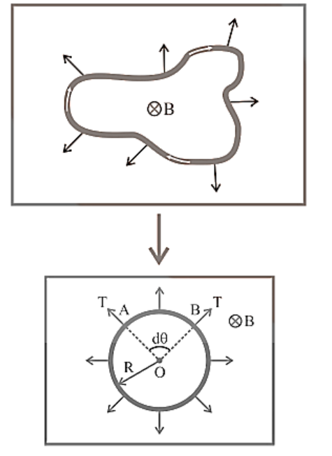
Force Experienced By An Arbitrary Current Carrying Loop In A Magnetic Field.
Specific example
In the above circular loop tension in parts A and B. In the balanced condition of small part AB of the loop is shown below
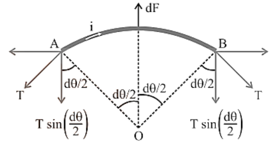
Force Experienced By A Small Part (Ab) Of An Arbitrary Current Carrying Loop In A Magnetic Field.
\[2{\text{T}}\sin \dfrac{{{\text{d}}\theta }}{2} = {\text{dF}} = {\text{Bid}}\ell \Rightarrow 2{\text{T}}\sin \dfrac{{{\text{d}}\theta }}{2} = {\text{BiRd}}\theta \]
If $d\theta $ is small so, \[\sin \dfrac{{{\text{d}}\theta }}{2} \approx \dfrac{{{\text{d}}\theta }}{2} \Rightarrow 2{\text{T}} \cdot \dfrac{{{\text{d}}\theta }}{2} = {\text{BiRd}}\theta \]
\[{\text{T}} = {\text{BiR}},{\text{if}}2\pi {\text{R}} = {\text{LsoT}} = \dfrac{{{\text{BiL}}}}{{2\pi }}\]
Note:
Even if there is no magnetic field, the loop will still widen into a circle because the current in its neighbouring sections is in the opposite direction, and opposing currents resist each other.
Case 2:
Equilibrium of a current-carrying conductor: A finite-length current-carrying wire can suspend freely in air when kept parallel to another infinite-length current-carrying wire, as shown below.
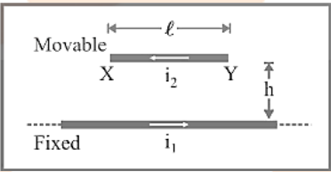
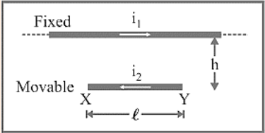
For XY equilibrium in both circumstances, downward weight = upward magnetic force, i.e.\[{\text{mg}} = \dfrac{{{\mu _0}}}{{4\pi }} \cdot \dfrac{{2{{\text{i}}_1}{{\text{i}}_2}}}{{\text{h}}} \cdot \ell \]’
Note:
If wire XY is slightly moved from its equilibrium position in the first example, SHM is executed, and the time duration is given by\[{\text{T}} = 2\pi \sqrt {\dfrac{{\text{h}}}{{\text{g}}}} \]
Case 3:
If a current-carrying straight wire is put in the magnetic field of a current-carrying circular loop, it creates a current-carrying circular loop.
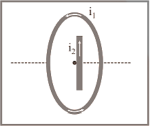
Due to the coil in its centre, the wire is positioned in a perpendicular magnetic field, causing it to feel maximum force \[{\text{F}} = {\text{Bi}}\ell = \dfrac{{{\mu _0}{{\text{i}}_1}}}{{2{\text{r}}}} \times {{\text{i}}_2}\ell \]
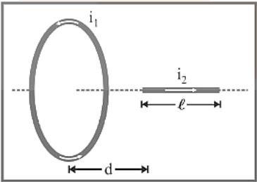
The wire is positioned parallel to the coil's axis, resulting in a magnetic field that is parallel to the wire. As a result, it will not be subjected to any force.
Case 4:
When current is passed through a spring, the spring contracts because the current flows in the same direction through all of the turns.
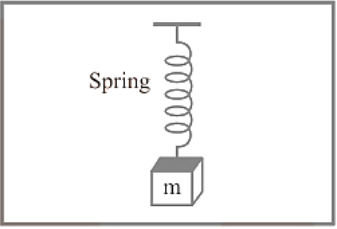
If current is allowed to flow through the spring, it will shrink and the weight will rise.
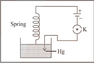
Case 5:
Tension-free strings: What is the value and direction of current via the conductor XY in the accompanying diagram such that the strings are tension-free?
If the weight of the conductor XY is balanced by magnetic force, the strings become tensionless (Fm)
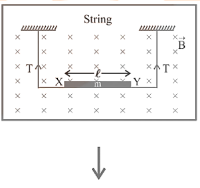
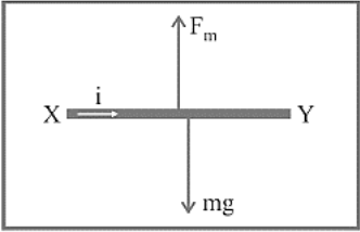
As a result, the current is flowing from X to Y and is in a balanced state.\[{{\text{F}}_{\text{m}}} = {\text{mg}} \Rightarrow {\text{Bi}}\ell = {\text{mg}} \Rightarrow {\text{i}} = \dfrac{{{\text{mg}}}}{{{\text{B}}\ell }}\]
Case 6:
A current-carrying conductor floating in air at an angle to the magnetic field's direction, while both the magnetic field and the conductor are on a horizontal plane.
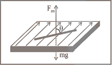
\[{\text{In equilibriummg}} = {\text{Bi}}\ell \sin \theta \Rightarrow {\text{i}} = \dfrac{{{\text{mg}}}}{{{\text{B}}\ell \sin \theta }}\]
Case 7:
Conducting rod sliding on inclined rails: When a conducting rod slides on inclined rails, it is said to be sliding.
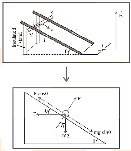
If a conducting rod (X, Y) moves at a constant velocity in the following condition,
\[{\text{F}}\cos \theta = {\text{mg}}\sin \theta \Rightarrow {\text{Bi}}\ell \cos \theta = {\text{mg}}\sin \theta \Rightarrow {\text{B}} = \dfrac{{{\text{mg}}}}{{{\text{i}}\ell }}\tan \theta \]
Tips and Tricks
1. The "Halmholtz galvanometer" is a gadget with a working principle based on Halmholtz coils and a homogeneous magnetic field.
2. Magnetic field induction is zero at the point where two linear parallel conductors carrying equal currents in the same direction meet in the middle of their separation.
3. When a current-carrying circular loop (n = 1) is wound into a coil with n identical turns, the magnetic field at the coil's centre is n2 times that of the preceding field, i.e.\[{{\text{B}}_{({\text{nturn}})}} = {{\text{n}}^2}{{\text{B}}_{({\text{single turn}})}}\]
4. The plane of a current-carrying coil hung freely in the earth's magnetic field remains East-West.
5. A moving charge q produces a magnetic field B, which is given by \[{\vec B} = \dfrac{{{\mu _0}}}{{4\pi }}\dfrac{{{\text{q}}({\vec v} \times {\vec r})}}{{{{\text{r}}^3}}} = \dfrac{{{\mu _0}}}{{4\pi }}\dfrac{{{\text{q}}({\vec v} \times {\text{\hat r}})}}{{{{\text{r}}^2}}}\] ; where v = velocity of charge and v < < c (speed of light).
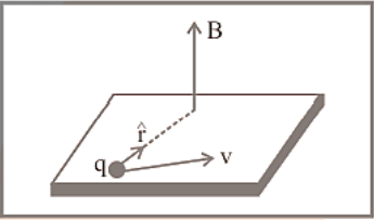
6. If an electron spins in a circular route with radius r and speed v, a magnetic field is created at the circular path's centre.\[{\text{B}} = \dfrac{{{\mu _0}}}{{4\pi }}\dfrac{{{\text{ev}}}}{{{{\text{r}}^2}}} \Rightarrow {\text{r}} \propto \sqrt {\dfrac{{\text{v}}}{{\text{B}}}} \].
7. Magnetomotive force is the line integral of the magnetising field H for any closed route (MMF). It’s SI unit is amp.
8. The dimension of the e.m.f. to the MMF ratio is the same as the dimension of resistance.
9. The ionisation of the gas produces positive ions in the space between the two dees. Hydrogen gas is utilised to make proton, whereas helium gas is used to make alpha particles.
10. Magnetic resonance frequency is another name for cyclotron frequency.
11. Because electrons have such a tiny mass, they cannot be accelerated by a cyclotron.
12. Because it encounters a force in a direction perpendicular to its velocity, the energy of a charged particle travelling in a homogeneous magnetic field remains unchanged. As a result, the charged particle's speed remains constant, and its K.E. remains constant.
13. When a charged particle is displaced by magnetic force, no work is done, while when the charged particle is moved by electric force, work is done.
14. The magnetic force is velocity dependent, whereas the electric force is unaffected by the charged particle's condition of rest or motion.
15. When a particle enters a magnetic field in a typical manner, it begins to move in a circular orbit. On the circumference is the point where it enters the magnetic field. (Most people confuse it with the orbit's centre.)
16. Charged particle deviation in magnetic field: If a charged particle (q, m) enters a uniform magnetic field B (which extends up to a length x) at right angles to the speed v as indicated in the picture. In a magnetic field, the particle's speed remains constant. In the magnetic field, Deviation in terms of time t: \[\theta = \omega {\text{t}} = \left( {\dfrac{{{\text{Bq}}}}{{\text{m}}}} \right){\text{t}}\]
Deviation in terms of length of the magnetic field ; \[\theta = {\sin ^{ - 1}}\left( {\dfrac{{\text{x}}}{{\text{r}}}} \right)\]
Only when $x \leqslant r$ is true can this relationship be employed.
The divergence will be 180° if x > r, as indicated in the diagram.
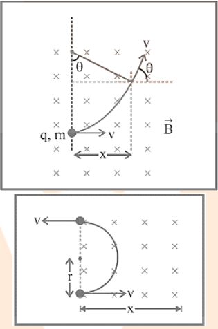
17. Even if there is no magnetic field, the loop will still widen into a circle because the current in its neighbouring sections is in the opposite direction, and opposing currents resist each other.
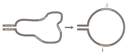
18. If wire XY is slightly moved from its equilibrium position in the following instance, SHM is executed, and the time duration is given by\[{\text{T}} = 2\pi \sqrt {\dfrac{{\text{h}}}{{\text{g}}}} \]
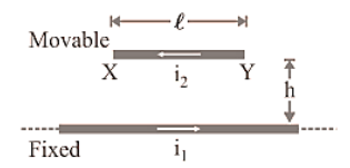
19. If the direction of current in the moveable wire is reversed in the preceding instance, the instantaneous acceleration generated is 2g$ \downarrow $.
20. For an observer, electric force is an absolute notion, whereas magnetic force is a relative one.
21. Electric force, as the dominator, determines the type of force between two parallel charge beams. Magnetic force determines the type of force between two parallel current-carrying wires.
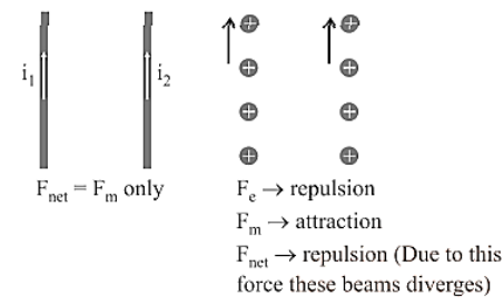
22. Because the magnetic field created by the coil is parallel to the wire, a straight current-carrying wire put along the axis of a current-carrying coil will not feel the magnetic force.
23. The force operating on a curved wire connecting points a and b in the picture is the same as the force acting on a straight wire connecting these locations. The phrase specifies it.\[\vec F = i\vec L \times \vec B\]
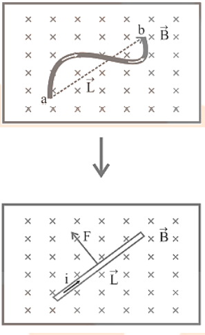
24. Force is created when a current-carrying conductor AB is positioned transverse to a long current-carrying conductor as illustrated.
Wire AB has a lot of experience.
\[{\text{F}} =\dfrac{{{\mu _0}{{\text{i}}_1}{{\text{i}}_2}}}{{2\pi }}{\log _{\text{e}}}\left( {\dfrac{{{\text{x}} +\ell }}{{\text{x}}}}\right)\]
Importance of Chapter 5 Magnetism and Matter Class 12 Notes
Foundation of Magnetism: This chapter lays the groundwork for understanding magnetic fields and forces, which are crucial for both academic study and real-world applications in physics.
Understanding Magnetic Properties: It explains the magnetic properties of different materials, helping you grasp how substances react in magnetic fields and the principles behind electromagnets and permanent magnets.
Key Concepts and Formulas: The notes cover important concepts such as magnetic field lines, the Earth's magnetic field, and the behavior of magnetic materials. Mastering these concepts is essential for solving problems and understanding advanced topics.
Real-World Applications: Knowledge from this chapter is applicable in various fields including engineering, electronics, and technology, making it relevant for practical applications and future studies.
Exam Preparation: The notes provide a structured overview of the chapter, making it easier to review and revise key topics. This helps in better preparation for exams and improves problem-solving skills.
Comprehensive Understanding: By studying this chapter, you'll gain a thorough understanding of how magnetism influences matter, which is fundamental for further studies in physics and related sciences.
Important Formulas of Class 12 Chapter 5 Physics You Shouldn’t Miss!
Here are the important formulas for Class 12 Physics Chapter 1: Magnetism and Matter that you shouldn’t miss:
1. Magnetic Field Due to a Long Straight Current-Carrying Wire:
\[B =\frac{\mu_0 I}{2 \pi r}\]
where \( B \) is the magnetic field, \( \mu_0 \) is the permeability of free space, \( I \) is the current, and \( r \) is the distance from the wire.
2. Magnetic Field Inside a Solenoid:
\[B =\mu_0 n I\]
where \( B \) is the magnetic field, \( \mu_0 \) is the permeability of free space, \( n \) is the number of turns per unit length, and \( I \) is the current.
3. Force on a Current-Carrying Wire in a Magnetic Field:
\[F = B I L \sin \theta\]
where \( F \) is the force, \( B \) is the magnetic field, \( I \) is the current, \( L \) is the length of the wire, and \( \theta \) is the angle between the wire and the magnetic field.
4. Magnetic Moment of a Current Loop:
\[\vec{m} = I A \hat{n}\]
where \( \vec{m} \) is the magnetic moment, \( I \) is the current, \( A \) is the area of the loop, and \( \hat{n} \) is the unit vector normal to the plane of the loop.
5. Torque on a Current Loop in a Magnetic Field:
\[\tau = m B \sin \theta\]
where \( \tau \) is the torque, \( m \) is the magnetic moment, \( B \) is the magnetic field, and \( \theta \) is the angle between the magnetic moment and the magnetic field.
6. Magnetic Field at the Center of a Circular Current Loop:
\[B =\frac{\mu_0 I}{2 R}\]
where \( B \) is the magnetic field, \( \mu_0 \) is the permeability of free space, \( I \) is the current, and \( R \) is the radius of the loop.
7. Magnetic Field Due to a Toroid:
\[B =\frac{\mu_0 N I}{2 \pi r}\]
where \( B \) is the magnetic field, \( \mu_0 \) is the permeability of free space, \( N \) is the number of turns, \( I \) is the current, and \( r \) is the radius of the toroid.
8. Gauss's Law for Magnetism:
\[\oint \vec{B} \cdot d\vec{A} = 0\]
This law states that the net magnetic flux through a closed surface is zero, indicating there are no magnetic monopoles.
Tips For Learning the Class 12 Physics Chapter 5 Magnetism and Matter
Here are some effective tips for learning Class 12 Physics Chapter 5: Magnetism and Matter:
Understand Basic Concepts: Start with the fundamental concepts of magnetism, including magnetic fields, forces, and the behavior of magnetic materials. Make sure you understand the definition and characteristics of magnetic fields and how they interact with matter.
Master Key Formulas: Memorize important formulas related to magnetic fields, forces, and moments. Practice applying these formulas to various problems to reinforce your understanding.
Use Visual Aids: Diagrams and illustrations can help visualize magnetic field lines, forces, and magnetic moments. Drawing these out or referring to textbook images can make concepts clearer.
Relate to Real-World Examples: Connect theoretical concepts with real-world applications such as electromagnets, MRI machines, and electric motors. Understanding how these concepts are used in practical situations can deepen your comprehension.
Solve Practice Problems: Work through a variety of problems from your textbook and other resources. This will help you apply theoretical knowledge to practical scenarios and prepare for exams.
Conclusion
Class 12 Physics Chapter 5: Magnetism and Matter explores the fundamental principles of magnetism and their applications in various scenarios. Understanding concepts such as magnetic fields, forces on current-carrying wires, and magnetic moments is crucial for mastering this chapter. By focusing on key formulas, using visual aids, and relating theoretical knowledge to practical examples, you can deepen your comprehension and enhance problem-solving skills. Consistent practice, review, and seeking help when needed will ensure a strong grasp of the material, helping you excel in both exams and real-world applications.
Important Magnetism and Matter Induction Related Links
Chapter-wise Links for Class 12 Physics Notes PDF FREE Download
Related Study Materials Links for Class 12 Physics
Along with this, students can also download additional study materials provided by Vedantu for Physics Class 12–