Alternating Current Class 12 Notes: CBSE Physics Chapter 7

Alternating Current

1. The Alternating Current

The magnitude of alternating current changes continuously with time and its direction is reversed periodically. It is represented by

${\text{I}} = {{\text{I}}_0}\sin \omega \,{\text{t}}$ or ${\text{I}} = {{\text{I}}_0}\cos \omega \,{\text{t}}$

$\omega  = \dfrac{{2\pi }}{{\text{T}}} = 2\pi {\text{v}}$

2. Average Value of Alternating Current

The mean or average value of alternating current over any half cycle is defined as that value of steady current which would send the same amount of charge through a circuit in the time of half cycle (i.e.${\text{T}}/2$) as is sent by the alternating current through the same circuit, in the same time.

To calculate the mean or average value, let an alternating current be represented by${\text{I}} = {{\text{I}}_0}\sin \omega \,{\text{t}}$    …(1)

If the strength of current is assumed to remain constant for a small time, ${\text{dt}}$, then small amount of charge sent in a small time dt is

${\text{dq}} = {\text{Idt}}$          …(2)

Let $q$ be the total charge sent by alternating current in the first half cycle (i.e. $0 \to {\text{T}}/2$).

$q = \int_0^{T/2} I dt$

${\text{U}}\operatorname{sing} (1)$, we get, ${\text{q}} = \int_0^{{\text{T}}/2} {{{\text{I}}_0}} \sin \omega {\text{t}} \cdot {\text{dt}} = {{\text{I}}_0}\left[ { - \dfrac{{\cos \omega {\text{t}}}}{\omega }} \right]_0^{{\text{T}}/2}$

$=  - \dfrac{{{{\text{I}}_0}}}{\omega }\left[ {\cos \omega \dfrac{{\text{T}}}{2} - \cos {0^o }} \right]$

 $=  - \dfrac{{{1_0}}}{\omega }\left[ {\cos \pi  - \cos {0^o }} \right]\quad (\because \omega {\text{T}} = 2\pi )$

${\text{q}} =  - \dfrac{{{{\text{I}}_0}}}{\omega }[ - 1 - 1] = \dfrac{{2{{\text{I}}_0}}}{\omega }$     …(3)

If ${I_m}$ represents the mean or average value of alternating current over the 1 st half cycle, then

${\text{q}} = {{\text{I}}_{\text{m}}} \times \dfrac{{\text{T}}}{2}$                      …(4)

From (3) and (4), we get ${{\text{I}}_{\text{m}}} \times \dfrac{{\text{T}}}{2} = 2\dfrac{{{{\text{I}}_0}}}{\omega } = \dfrac{{2{{\text{I}}_0} \cdot {\text{T}}}}{{2\pi }}$     …(5)

or $\quad {I_m} = \dfrac{2}{\pi }{I_0} = 0.637{{\text{I}}_0}$

Hence, the mean or average value of alternating current over the positive half cycle is 0.637 times the peak value of alternating current, i.e., $63.7\% $ of the peak value.

3. A.C. Circuit Containing Resistance Only

Let a source of alternating e.m.f. be connected to a pure resistance R, Figure. Suppose the alternating e.m.f. supplied is represented by

$E = {E_0}\sin \omega t$     …(1)

Let $I$ be the current in the circuit at any instant $t$. The potential difference developed across ${\text{R}}$ will be IR. This must be equal to e.m.f. applied at that instant, i.e., ${\text{IR}} = E = {E_0}\sin \omega t$

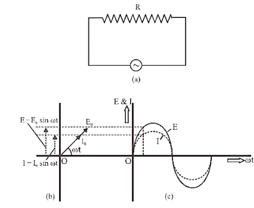
or $\quad I = \dfrac{{{E_0}}}{R}\sin \omega t = {I_0}\sin \omega t$        …(2)

where ${I_0} = {E_0}/R$, maximum value of current.

This is the form of alternating current developed.

Comparing ${{\text{I}}_0} = {{\text{E}}_0}/{\text{R}}$ with Ohm's law equation, viz. current = voltage/resistance, we find that resistance to a.c. is represented by R-which is the value of resistance to ${\text{d}}$.c. Hence behaviour of ${\text{R}}$ in d.c. and a.c. circuit is the same, ${\text{R}}$ can reduce a.c. as well as d.c. equally effectively.

Comparing (2) and (1), we find that $E$ and I are in phase. Therefore, in an a.c. circuit containing $R$ only, the voltage and current are in the same phase, as shown in figure.

3.1 Phasor Diagram

In the a.c. circuit containing $R$ only, current and voltage are in the same phase. Therefore, in figure, both phasors ${\overrightarrow {\text{I}} _0}$ and ${\overrightarrow {\text{E}} _0}$ are in the same direction making an angle $(\omega {\text{t}})$ with OX. This is so for all times. It means that the phase angle between alternating voltage and alternating current through ${\text{R}}$ is zero.

${\text{I}} = {{\text{I}}_0}\sin \omega {\text{t}}$ and ${\text{E}} = {{\text{E}}_0}\sin \omega {\text{t}}$

4. A.C. Circuit Containing Inductance Only

In an a.c. circuit containing $L$ only alternating current $I$ lags behind alternating voltage $E$ by a phase angle of ${90^o }$, i.e., by one fourth of a period. Conversely, voltage across L leads the current by a phase angle of ${90^o }$. This is shown in figure.

Figure (b) represents the vector diagram or the phasor diagram of a.c. circuit containing $L$ only. The vector representing ${\vec E_0}$ makes an angle ($\omega t$) with OX. As current lags behind the e.m.f. by ${90^o }$, therefore, phasor representing ${\vec I_0}$ is turned clockwise through ${90^o }$ from the direction of

${\overrightarrow {\text{E}} _0}.{\text{I}} = {{\text{I}}_0}\sin \left( {\omega {\text{t}} - \dfrac{\pi }{2}} \right),{{\text{I}}_0} = \dfrac{{{{\text{v}}_0}}}{{{{\text{x}}_{\text{L}}}}},{{\text{X}}_{\text{L}}} = \omega {\text{L}}$

A pure inductance offers zero resistance to dc. It means a pure inductor cannot reduce dc. The units of inductive reactance

${{\text{X}}_{\text{L}}} = \omega L \Rightarrow \dfrac{1}{{{\text{sec}}}}({\text{ henry }}) = \dfrac{1}{{{\text{sec}}}}\dfrac{1}{{{\text{amp}}/{\text{sec}}}} = {\text{ohm}}$

The dimensions of inductive reactance are the same as those of resistance.

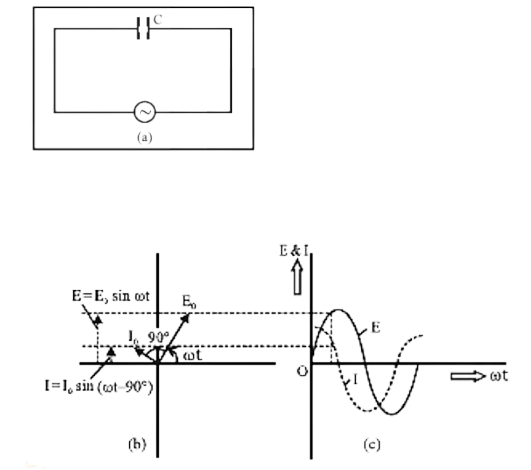
5. A.C. Circuit Containing Capacitance Only

Let a source of alternating e.m.f. be connected to a capacitor only of capacitance $C$, figure. Suppose the alternating e.m.f. supplied is

$E = {E_0}\sin \omega t$            …(1)

The current flowing in the circuit transfers charge to the plates of the capacitor. This produces a potential difference between the plates. The capacitor is alternately charged and discharged as the current reverses each half cycle. At any instant $t$, suppose $q$ is the charge on the capacitor. Therefore, potential difference across the plates of capacitor ${\text{V}} = {\text{q}}/{\text{C}}$.

At every instant, the potential difference V must be equal to the e.m.f. applied i.e.,

${\text{V}} = \dfrac{{\text{q}}}{{\text{C}}} = {\text{E}} = {{\text{E}}_0}\sin \omega {\text{t}}$

Or  ${\text{q}} = {\text{C}}{\varepsilon _0}\sin \omega {\text{t}}$

If I is instantaneous value of current in the circuit at instant ${\text{t}}$, then

$I = \dfrac{{dq}}{{dt}} = \dfrac{d}{{dt}}\left( {C{\varepsilon _0}\sin \omega t} \right)$

$I = C{E_0}(\cos \omega t)\omega$

$I = \dfrac{{{E_0}}}{{1/\omega C}}\sin (\omega t + \pi /2)$                …(2)

The current will be maximum i.e.,

$I = {I_0}$, when $\sin (\omega t + \pi /2) = $ maximum $ = 1$

$\therefore \quad $ From $(2),{I_0} = \dfrac{{{E_0}}}{{1/\omega C}} \times 1$         …(3)

Put in (2), ${\text{I}} = {{\text{I}}_0}\sin (\omega {\text{t}} + \pi /2)$     …(4)

This is the form of alternating current developed.

Comparing (4) with (1), we find that in an a.c. circuit containing C only, alternating current leads the alternating e.m.f. by a phase angle of ${90^o }$. This is shown in figure (b) and (c).

The phasor diagram or vector diagram of a.c. circuit containing C only in shown in figure (b). The phasor ${\vec I_0}$ is turned anticlockwise through ${90^o }$ from the direction of phasor ${\vec E_0}$. Their projections on ${\text{YO}}{{\text{Y}}^\prime }$ give the instantaneous values ${\text{E}}$ and $I$ as shown in figure (b). When ${E_0}$ and ${I_0}$ rotate with frequency $\omega $, curves in figure (c). are generated.

Comparing (3) with Ohm's law equation, viz current = voltage/resistance, we find that $(1/\omega C)$ represents effective resistance offered by the capacitor. This is called capacitive reactance and is denoted by ${{\text{X}}_{\text{c}}}$,

Thus, ${{\text{X}}_{\text{C}}} = \dfrac{1}{{\omega {\text{C}}}} = \dfrac{1}{{2\pi {\text{VC}}}}$

The capacitive reactance limits the amplitude of current in a purely capacitive circuit in the same way as the resistance limits the current in a purely resistive circuit. Clearly, capacitive reactance varies inversely as the frequency of a.c. and also inversely as the capacitance of the condenser.

In a d.c. circuit, ${\text{v}} = 0,\therefore {\text{XC}} = \infty $

${{\text{X}}_{\text{c}}} = \dfrac{1}{{\omega {\text{C}}}} = \sec \dfrac{1}{{{\text{ farad }}}} = \dfrac{{{\text{sec}}}}{{{\text{ coulomb/ volt }}}}$

${{\text{X}}_{\text{c}}}\, = \dfrac{{{\text{ voltsec}}{\text{. }}}}{{{\text{ amp}}{\text{.sec }}}} = {\text{olm}}$

5. A.C. Circuit Containing Resistance, Inductance and Capacitance and Series

6.1 Phasor Treatment

Let a pure resistance $R$, a pure inductance $L$ and an ideal capacitor of capacitance ${\text{C}}$ be connected in series to a source of alternating e.m.f. figure. As ${\text{R}},{\text{L}},{\text{C}}$ are in series, therefore, current at any instant through the three elements has the same amplitude and phase. Let it be represented by ${\text{I}} = {{\text{I}}_0}\sin \omega {\text{t}}$

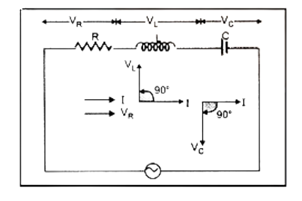
However, voltage across each element bears a different phase relationship with the current. Now,

(i) The maximum voltage across ${\text{R}}$ is

${\overrightarrow {\text{V}} _{\text{R}}} = {\overrightarrow {\text{I}} _0}{\text{R}}$

In figure, the current phasor ${\vec I_0}$ is represented along ${\text{OX}}$.

As ${\vec V_R}$ is in phase with current, it is represented by the vector $\overrightarrow {{\text{OA}}} $, along ${\text{OX}}$.

(ii) The maximum voltage across ${\text{L}}$ is ${\overrightarrow {\text{V}} _{\text{L}}} = {\overrightarrow {\text{I}} _0}{{\text{X}}_{\text{L}}}$

As voltage across the inductor leads the current by ${90^o }$, it is represented by $\overrightarrow {{\text{OB}}} $ along ${\text{OY}},{90^o }$ ahead of ${\overrightarrow {\text{I}} _0}$.

(iii) The maximum voltage across ${\text{C}}$ is ${\overrightarrow {\text{V}} _{\text{C}}} = {\overrightarrow {\text{I}} _0}{{\text{X}}_{\text{C}}}$

As voltage across the capacitor lags behind the alternating current by ${90^o }$, it is represented by $\overrightarrow {{\text{OC}}} $ rotated clockwise through ${90^o }$ from the direction of ${\vec I_0} \cdot \overrightarrow {OC} $ is along $O{{\text{Y}}^\prime }$

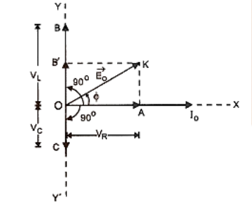
6.2 Analytical Treatment of RLC Series Circuit

Let a pure resistance ${\text{R}}$, a pure inductance ${\text{L}}$ and an ideal condenser of capacity ${\text{C}}$ be connected in series to a source of alternating e.m.f. Suppose the alternating e.m.f. supplied is

${\text{E}} = {{\text{E}}_0}\sin \omega {\text{t}}$    …(1)

At any instant of time t, suppose

$q = $ charge on capacitor

${\text{I}} = $ current in the circuit

$\dfrac{{{\text{dI}}}}{{{\text{dt}}}} = $ rate of change of current in the circuit

potential difference across the condenser $ = \dfrac{q}{C}$

potential difference across inductor $ = {\text{L}}\dfrac{{{\text{dI}}}}{{{\text{d}}t}}$

potential difference across resistance $ = {\text{RI}}$

$\therefore $ The voltage equation of the circuit is

${\text{L}}\dfrac{{{\text{dI}}}}{{{\text{dt}}}} + {\text{RI}} + \dfrac{{\text{q}}}{{\text{C}}} = {\text{E}} = {{\text{E}}_0}\sin \omega {\text{t}}$          …(2)

As $I = \dfrac{{dq}}{{dt}}$, therefore, $\dfrac{{dI}}{{dt}} = \dfrac{{{d^2}q}}{{d{t^2}}}$

$\therefore $ The voltage equation becomes

${\text{L}}\dfrac{{{{\text{d}}^2}{\text{q}}}}{{{\text{d}}{{\text{t}}^2}}} + {\text{R}}\dfrac{{{\text{dq}}}}{{{\text{dt}}}} + \dfrac{{\text{q}}}{{\text{C}}} = {{\text{E}}_0}\sin \omega {\text{t}}$           …(3)

This is like the equation of a forced, damped oscillator. Let the solution of equation (3) be

$q = {q_0}\sin (\omega t + \theta )$

$\therefore \quad \dfrac{{dq}}{{dt}} = {q_0}\omega \cos (\omega t + \theta )$

 $\dfrac{{{d^2}q}}{{d{t^2}}} =  - {q_0}{\omega ^2}\sin (\omega t + \theta )$

Substituting these values in equation (3), we get 

$L\left[ { - {q_0}{\omega ^2}\sin (\omega t + \theta )} \right] + R{q_0}\omega \cos (\omega t + \theta )$

$\dfrac{{{q_0}}}{C}\sin (\omega t + \theta ) = {E_0}\sin \omega t$  ${q_0}\omega \left[ {R\cos (\omega t + \theta ) - \omega L\sin (\omega t + \theta ) + \dfrac{1}{{\omega C}}\sin \left( {\omega t + \theta } \right)} \right] = {E_0}\sin \omega t$

As ${\omega _{\text{L}}} = {{\text{X}}_{\text{L}}}$ and $\dfrac{1}{{{\text{OC}}}} = {{\text{X}}_{\text{C}}}$, therefore ${q_0}\omega \left[ {R\cos (\omega t + \theta ) + \left( {{X_C} - {X_L}} \right)\sin (\omega t + \theta )} \right] = {E_0}\sin \omega t$ Multiplying and dividing by,

$Z = \sqrt {{R^2} + {{\left( {{X_C} - {X_L}} \right)}^2}} $, we get

${q_0}\omega Z\left[ {\dfrac{R}{Z}\cos (\omega t + \theta ) + \dfrac{{{X_C} - {X_L}}}{Z}\sin (\omega t + \theta )} \right] = {E_0}\sin \omega t$        …(4)

Let $\dfrac{{\text{R}}}{Z} = \cos \phi $ and $\dfrac{{{{\text{X}}_{\text{C}}} - {{\text{X}}_{\text{L}}}}}{{\text{Z}}} = \sin \phi $                  …(5)

So that $\tan \phi  = \dfrac{{{X_c} - {X_L}}}{Z}$                                    …(6)

$\therefore \,{q_0}\omega Z\left[ {\cos \left( {\omega t + \theta } \right)\cos \phi  + \sin \left( {\omega t + \theta } \right)\sin \phi } \right] = {E_0}\sin \omega t$

or $\quad {q_0}\omega Z\cos (\omega t + \theta  - \phi ) = {E_0}\sin \omega t = {E_0}\cos (\omega t - \pi /2)\quad  \ldots (7)$

Comparing the two sides of this equation, we find that ${E_0} = {q_0}\omega Z = {I_0}Z$, where ${I_0}{q_0}\omega $  …(8)

and $\omega t + \theta  - \phi  = \omega t - \pi /2$

$\therefore \,\,\theta  - \phi  = \dfrac{{ - \pi }}{2}$ 

or $\theta  = \dfrac{{ - \pi }}{2} + \phi $                   …(9)

Current in the circuit is

$I = \dfrac{{dq}}{{dt}} = \dfrac{d}{{dt}}\left[ {{q_0}\sin (\omega t + \theta )} \right] = {q_0}\omega \cos (\omega t + \theta )$ 

$I = {I_0}\cos (\omega t + \theta )\quad \{ {\text{ using }}(8)\}$  

Using $(9)$, we get, ${\text{I}} = {{\text{I}}_0}\cos (\omega {\text{t}} + \phi  - \pi /2)$

${\text{I}} = {{\text{I}}_0}\sin (\omega {\text{t}} + \phi )$               …(10)

${\text{From }}(6),\phi  = {\tan ^{ - 1}}\dfrac{{\left( {{{\text{X}}_{\text{C}}} - {{\text{X}}_{\text{L}}}} \right)}}{{\text{R}}}$        …(11)

As ${\cos ^2}\phi  + {\sin ^2}\phi  = 1$

$\therefore \,\,{\left( {\dfrac{R}{Z}} \right)^2} + {\left( {\dfrac{{{X_C} - {X_L}}}{Z}} \right)^2} = 1$

${R_2} + {\left( {{X_C} - {X_L}} \right)^2} = {Z^2}$

$Z = \sqrt {{R^2} + {{\left( {{X_C} - {X_L}} \right)}^2}} $                  …(12)

7. A.C. Circuit containing Resistance & Inductance

Let a source of alternating e ${\text{m}}$ f be connected to an ohmic resistance ${\text{R}}$ and a coil of inductance $L$, in series as shown in figure.

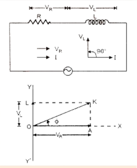
$Z = \sqrt {{R^2} + X_L^2} $

We find that in RL circuit, voltage leads the current by a phase angle $\phi $, where

$\tan \phi  = \dfrac{{{\text{AK}}}}{{{\text{OA}}}} = \dfrac{{{\text{OL}}}}{{{\text{OA}}}} = \dfrac{{{{\text{V}}_{\text{L}}}}}{{{{\text{V}}_{\text{R}}}}} = \dfrac{{{{\text{I}}_0}{{\text{X}}_{\text{L}}}}}{{{{\text{I}}_0}{\text{R}}}}$

$\tan \phi  = \dfrac{{{{\text{X}}_{\text{L}}}}}{{\text{R}}}$

8. A.C. Circuit Containing Resistance and Capacitance

Let a source of alternating e.m.f. be connected to an ohmic resistance ${\text{R}}$ and a condenser of capacity ${\text{C}}$, in series as shown in figure.

$Z = \sqrt {{R^2} + X_C^2} $

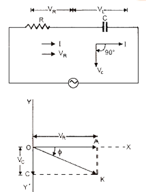
Figure represents phasor diagram of ${\text{RC}}$ circuit. We find that in RC circuit, voltage lags behind the current by a phase angle $\phi $, where

$\tan \phi  = \dfrac{{AK}}{{OA}} = \dfrac{{OC}}{{OA}} = \dfrac{{{V_C}}}{{{V_R}}} = \dfrac{{{I_0}{X_C}}}{{{I_0}R}}$

$\tan \phi  = \dfrac{{{X_C}}}{R}$

9. Energy Stored in an Inductor

When a.c. is applied to an inductor of inductance ${\text{L}}$, the current in it grows from zero to maximum steady value ${{\text{I}}_0}$ If ${\text{I}}$ is the current at any instant ${\text{t}}$, then the magnitude of induced e ${\text{m}}$.f. developed in the inductor at that instant is,

${\text{E}} = {\text{L}}\dfrac{{{\text{dI}}}}{{{\text{dt}}}}$                   …(1)

The self induced e.m.f. is also called the back e.m.f., as it opposes any change in the current in the circuit.

Physically, the self inductance plays the role of inertia. It is the electromagnetic analogue of mass in mechanics. Therefore, work needs to be done against the back e.m.f. $E$. in establishing the current. This work is stored in the inductor as magnetic potential energy.

For the current $I$ at an instant $t$, the rate of doing work is,

$\dfrac{{{\text{dW}}}}{{{\text{dt}}}} = {\text{EI}}$

If we ignore the resistive losses, and consider only inductive effect, then

Using $(1),\dfrac{{{\text{dW}}}}{{{\text{dt}}}} = {\text{EI}} = {\text{L}}\dfrac{{{\text{dI}}}}{{{\text{dt}}}} \times {\text{I}}$ or ${\text{dW}} = {\text{LIdI}}$

Total amount of work done in establishing the current I is,

${\text{W}} = \int {{\text{dW}}}  = \int_0^1 {\;{\text{L}}} I\;{\text{dI}} = \dfrac{1}{2}{\text{L}}{{\text{I}}^2}$

Thus energy required to build up current in an inductor = energy stored in inductor,

${{\text{U}}_{\text{B}}} = {\text{W}} = \dfrac{1}{2}{\text{L}}{{\text{I}}^2}$

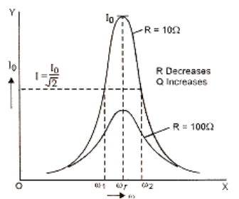
10. Electric Resonance

10.1 Series Resonance Circuit

A circuit in which inductance $L$, capacitance $C$ and resistance ${\text{R}}$ are connected in series, and the circuit admits maximum current corresponding to a given frequency of a.c., is called series resonance circuit.

The impedance (Z) of an RLC circuit is given by

$Z = \sqrt {{R^2} + {{\left( {\omega L - \dfrac{1}{{\omega C}}} \right)}^2}} $                 …(1)

At very low frequencies, inductive reactance ${{\text{X}}_{\text{L}}} = \omega {\text{L}}$ is negligible, but capacitive reactance $\left( {{{\text{X}}_{\text{C}}} = 1/\omega {\text{C}}} \right)$ is very high.

As frequency of alternating e.m.f. applied to the circuit is increased, ${X_1}$ goes on increasing and ${X_c}$ goes on decreasing. For a particular value of $\omega \left( { = {\omega _t}} \right.$, say )

${{\text{X}}_{\text{L}}} = {{\text{X}}_{\text{c}}}$

i.e., ${\omega _r}\;{\text{L}} = \dfrac{1}{{{\omega _{\text{r}}}{\text{C}}}}$ or ${\omega _{\text{r}}} = \dfrac{1}{{\sqrt {{\text{LC}}} }}$

$2\pi {{\text{v}}_{\text{r}}} = \dfrac{1}{{\sqrt {{\text{LC}}} }}{\text{ or }}{{\text{v}}_{\text{r}}} = \dfrac{1}{{2\pi \sqrt {{\text{LC}}} }}$

At this particular frequency ${v_f}$ as ${{\text{X}}_{\text{L}}} = {{\text{X}}_{\text{c}}}$, therefore, from (1)

$Z = \sqrt {{R^2} + 0}  = R = \operatorname{minimum} $

i.e. impedance of RLC circuit is minimum and hence the current ${I_0} = \dfrac{{{E_0}}}{Z} = \dfrac{{{E_0}}}{R}$ becomes maximum. This frequency is called series resonance frequency.

The $Q$ factor of a series resonant circuit is defined as the ratio of the voltage developed across the inductance or capacitance at resonance to the impressed voltage, which is the voltage applied across $R$.

i.e.,

${\text{i}}{\text{.e}}{\text{. }}\quad Q = \dfrac{{{\text{ voltage across }}L{\text{ or }}C}}{{{\text{ applied voltage ( =  voltage across R ) }}}}$

  $Q = \dfrac{{\left( {{\omega _r}\;{\text{L}}} \right)I}}{{{\text{RI}}}} = \dfrac{{{\omega _{\text{r}}}{\text{L}}}}{{\text{R}}}{\text{ }}$

  ${\text{or }}\quad {\text{Q}} = \dfrac{{\left( {1/{\omega _{\text{r}}}{\text{C}}} \right){\text{I}}}}{{{\text{RI}}}} = \dfrac{{\text{I}}}{{{\text{RC}}{\omega _{\text{r}}}}}$

Using ${\omega _r} = \dfrac{1}{{\sqrt {{\text{LC}}} }}$, we get

${\text{Q}} = \dfrac{{\text{L}}}{{\text{R}}}\dfrac{1}{{\sqrt {{\text{LC}}} }} = \dfrac{1}{{\text{R}}}\sqrt {\dfrac{{\text{L}}}{{\text{C}}}} $

or $\quad Q = \dfrac{{1\sqrt {LC} }}{{RC}} = \dfrac{1}{R}\sqrt {\dfrac{L}{C}} $

Thus $Q = \dfrac{1}{R}\sqrt {\dfrac{L}{C}} $                      …(1)

The quantity $\left( {\dfrac{{{\omega _r}}}{{2\Delta \omega }}} \right)$ is regarded as a measure of the sharpness of resonance, i.e., $Q$ factor of the resonance circuit is the ratio of resonance angular frequency to bandwidth of the circuit (which is a difference in angular frequencies at which power is half the maximum power or current is ${{\text{I}}_0}/\sqrt 2 $.

10.2 Average Power in RLC circuit or Inductive Circuit

Let the alternating e.m.f. applied to an RLC circuit be,

$E = {E_0}\sin \omega t$                …(1)

If alternating current developed lags behind the applied e.m.f. by a phase angle $\phi $, then

${\text{I}} = {{\text{I}}_0}\sin (\omega {\text{t}} - \phi )$          …(2)

Power at instant t, $\dfrac{{{\text{dW}}}}{{{\text{dt}}}} = {\text{EI}}$

$\dfrac{{{\text{dW}}}}{{{\text{dt}}}} = {{\text{E}}_0}\sin \omega {\text{t}} \times {{\text{I}}_0}\sin (\omega {\text{t}} - \phi )$

$ = {{\text{E}}_0}{{\text{I}}_0}\sin \omega {\text{t}}(\sin \omega {\text{cos}}\phi  - \cos \omega {\text{sin}}\phi )$

$ = {{\text{E}}_0}{{\text{I}}_0}{\sin ^2}\omega \cos \phi  - {{\text{E}}_0}{{\text{I}}_0}\sin \omega \cos \omega \sin \phi $

$ = {{\text{E}}_0}{{\text{I}}_0}{\sin ^2}\omega t\cos \phi  - \dfrac{{{{\text{E}}_0}{{\text{I}}_0}}}{2}\sin 2\omega {\text{sin}}\phi $

If this instantaneous power is assumed to remain constant for a small time $dt$, then small amount of work done in this time is.

${\text{dW}} = \left( {{{\text{E}}_0}{{\text{I}}_0}{{\sin }^2}\omega {\text{t}}\cos \phi  - \dfrac{{{{\text{E}}_0}{{\text{I}}_0}}}{2}\sin 2\omega {\text{sin}}\phi } \right){\text{dt}}$

Total work done over a complete cycle is

${\text{W}} = \int_0^{\text{T}} {{{\text{E}}_0}} {{\text{I}}_0}{\sin ^2}\omega t\cos \phi {\text{dt}} - \int_0^T {\dfrac{{{{\text{E}}_0}{{\text{I}}_0}}}{2}} \sin 2\omega {\text{sin}}\phi {\text{dt}}$

${\text{W}} = {{\text{E}}_0}{{\text{I}}_0}\cos \phi \int_0^{\text{T}} {{{\sin }^2}} \omega {\text{dt}} - \dfrac{{{{\text{E}}_0}{{\text{I}}_0}}}{2}\sin \phi \int_0^{\text{T}} {\sin } 2\omega {\text{tdt}}$

As $\int_0^{\text{T}} {{{\sin }^2}} \omega {\text{td}} = \dfrac{{\text{T}}}{2}$ and $\int_0^{\text{T}} {\sin } \omega {\text{tdt}} = 0$

$\therefore \quad {\text{W}} = {E_0}{I_0}\cos \phi  \times \dfrac{T}{2}$

$\therefore \quad $ Average power in the inductive circuit over a complete cycle.

$P = \dfrac{W}{T} = \dfrac{{{E_0}{I_0}\cos \phi }}{T} \cdot \dfrac{T}{2} = \dfrac{{{E_0}}}{{\sqrt 2 }}\dfrac{{{I_0}}}{{\sqrt 2 }}\cos \phi $

$P = {E_v}{I_v}\cos \phi $                                  …(3)

Hence average power over a complete cycle in an inductive circuit is the product of virtual e.m.f., virtual current and cosine of the phase angle between the voltage and current.

Note:

The relation (3) is applicable to all a.c. circuits. $\cos \phi $ and $Z$ will have appropriate values for different circuits.

For example:

(i) In PL circuit, $Z = \sqrt {{R^2} + X_L^2} $ and $\cos \phi  = \dfrac{R}{Z}$

(ii) $\operatorname{In} {\text{RC}}$ circuit, $Z = \sqrt {{{\text{R}}^2} + {\text{X}}_{\text{C}}^2} $ and $\cos \phi  = \dfrac{{\text{R}}}{{\text{Z}}}$

(iii) In LC circuit, ${\text{Z}} = {{\text{X}}_{\text{L}}} - {{\text{X}}_{\text{c}}}$ and $\phi  = {90^o }$

(iv) In RLC circuit, ${\text{Z}} = \sqrt {{{\text{R}}^2} + {{\left( {{{\text{X}}_{\text{L}}} - {{\text{X}}_{\text{C}}}} \right)}^2}} $ and $\cos \phi  = \dfrac{{\text{R}}}{{\text{Z}}}$

In all a.c. circuits, ${I_v} = \dfrac{{{E_v}}}{Z}$

10.3 Power Factor of an A.C. Circuit

We have proved that average power/cycle in an inductive circuit is

$P = {E_v}{I_v}\cos \phi $             …(1)

Here, P is called true power, $\left( {{E_V},\,{I_V}} \right)$ is called apparent power or virtual power and$\cos \phi $ is called power factor of the circuit.

Thus, Power factor $ = \dfrac{{{\text{ true power }}({\text{P}})}}{{{\text{ apparent power }}\left( {{{\text{E}}_{\text{v}}}{{\text{I}}_{\text{v}}}} \right)}} = \cos \phi $         …(2)

$ = \dfrac{{\text{R}}}{{\sqrt {{{\text{R}}^2} + {{\left( {{{\text{X}}_{\text{L}}} - {{\text{X}}_{\text{C}}}} \right)}^2}} }}\quad [$ from impedance triangle]

Power factor $ = \cos \phi  = \dfrac{{{\text{ Resistance }}}}{{{\text{ Impedance }}}}$

In a non-inductance circuit, ${{\text{X}}_{\text{L}}} = {{\text{X}}_{\text{C}}}$

$\therefore \quad $ Power factor $ = \cos \phi  = \dfrac{{\text{R}}}{{\sqrt {{{\text{R}}^2}} }} = \dfrac{{\text{R}}}{{\text{R}}} = 1,\phi  = {0^o }$

This is the maximum value of power factor. In a pure inductor or an ideal capacitor, $\phi  = {90^o }$.

Power factor $ = \cos \phi  = \cos {90^o } = 0$.

Average power consumed in a pure inductor or ideal a capacitor, ${\text{P}} = {{\text{E}}_v}{I_{\text{y}}}\cos {90^o } = $ Zero. Therefore, current through pure ${\text{L}}$ or pure ${\text{C}}$, which consumes no power for its maintenance in the circuit is called Idle current or Watt less current.

In actual practice, we do not have an ideal inductor or ideal capacitor. Therefore, there does occur some dissipation of energy. However, inductance and capacitance continue to be most suitable for controlling current in a.c. circuits with minimum loss of power.

12. Transformer

A transformer which increases the a.c. voltage is called a step-up transformer. A transformer which decreases the a.c. voltages are called a step-down transformer.

12.1 Principle

A transformer is based on the principle of mutual induction, i.e., whenever the amount of magnetic flux linked with a coil changes, an e.m.f. is induced in the neighbouring coil.

12.2 Construction

A transformer consists of a rectangular soft iron core made of laminated sheets, well insulated from one another, figure. Two coils ${{\text{P}}_1}{{\text{P}}_2}$ (the primary coil) and ${{\text{S}}_1}\;{{\text{S}}_2}$ (the secondary coil) are wound on the same core, but are well insulated from each other. Note that both the coils are also insulated from the core. The source of alternating e.m.f. (to be transformed) is connected to the primary coil ${{\text{P}}_1}{{\text{P}}_2}$ and a load resistance $R$ is connected to the secondary coil ${{\text{S}}_1}\;{{\text{S}}_2}$ through an open switch ${\text{S}}$. Thus, there can be no current through the secondary coil so long as the switch is open.

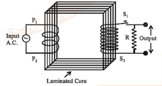
For an ideal transformer, we assume that the resistances of the primary and secondary windings are negligible.

Further, the energy losses due to magnetic hysteresis in the iron core is also negligible. Well-designed high capacity transformers may have energy losses as low as $1\% $.

12.3 Theory and Working

Let the alternating e.m.f. supplied by the a.c. source connected to primary be

${E_p} = {E_0}\sin \omega t$                    …(1)

As we have assumed the primary to be a pure inductance with zero resistance, the sinusoidal primary current ${{\text{I}}_{\text{p}}}$ lags the primary voltage ${E_p}$ by ${90^o }$. The primary's power factor, $\cos \phi  = {90^o } = 0.$ Therefore, no power is dissipated in primary.

The alternating primary current induces an alternating magnetic flux ${\phi _{\text{B}}}$ in the iron core. Because the core extends through the secondary winding, the induced flux also extends through the turns of the secondary.

According to Faraday's law of electromagnetic induction. the induced e.m.f. per turn $\left( {{E_{{\text{tro }}}}} \right)$ is same for both, the primary and secondary. Also, the voltage ${E_p}$ across the primary is equal to the e.m.f. induced in the primary, and the voltage ${E_s}$ across the secondary is equal to the e.m.f. induced in the secondary. Thus,

${E_{{\text{tum }}}} = \dfrac{{d{\phi _B}}}{{dt}} = \dfrac{{{E_p}}}{{{n_p}}} = \dfrac{{{E_s}}}{{{n_s}}}$

Here, ${n_p};{n_s}$ represent total number of tums in primary and secondary coils respectively-

${E_a} = {E_p}\dfrac{{{n_a}}}{{{n_p}}}$                           …(2)

If ${n_s} > {n_p};{E_s} > {E_p}$, the transformer is a step up transformer. Similarly, when ${n_s} < {n_p};{E_s} < {E_p}.$ The device is called a step down transformer. $\dfrac{{{{\text{n}}_{\text{s}}}}}{{{{\text{n}}_{\text{p}}}}} = {\text{K}}$ represents transformation ratio.

Note that this relation (2) is based on three assumptions

(i) the primary resistance and current are small,

(ii) there is no leakage of magnetic flux. The same magnetic flux links both, the primary and secondary coil,

(iii) the secondary current is small.

Now, the rate at which the generator/source transfer energy to the primary $ = {{\text{I}}_{\text{p}}}{{\text{E}}_{\text{p}}}.$ The rate at which the primary then transfers energy to the secondary (via the alternating magnetic field linking the two coils) is ${{\text{I}}_{\text{s}}}{{\text{E}}_{\text{s}}}$.

As we assume that no energy is lost along the way, conservation of energy requires that

${{\text{I}}_{\text{p}}}{{\text{E}}_{\text{p}}}{\text{ = }}{{\text{I}}_{\text{s}}}{{\text{E}}_{\text{s}}}$

$\therefore {{\text{I}}_{\text{s}}}{\text{ = }}{{\text{I}}_{\text{p}}}\dfrac{{{{\text{E}}_{\text{p}}}}}{{{{\text{E}}_{\text{s}}}}}$

From (2), 

$\dfrac{{{{\text{E}}_{\text{p}}}}}{{{{\text{E}}_{\text{s}}}}}{\text{ = }}\dfrac{{{{\text{n}}_{\text{p}}}}}{{{{\text{n}}_{\text{s}}}}}$

$\therefore \,\,\,\,{{\text{I}}_{\text{s}}}{\text{ =  }}{{\text{I}}_{\text{p}}}\dfrac{{{{\text{n}}_{\text{P}}}}}{{{{\text{n}}_{\text{s}}}}}{\text{ = }}\dfrac{{{{\text{I}}_{\text{p}}}}}{{\text{K}}}$               …(3)

For a step up transformer, ${E_s} > {E_p};K > 1\therefore {I_s} < {I_p}$ i.e. secondary current is weaker when secondary voltage is higher, i.e., whatever we gain in voltage, we lose in current in the same ratio.

The reverse is true for a step-down transformer.

From eqn. (3) ${I_p} = {I_s}\left( {\dfrac{{{n_s}}}{{{n_p}}}} \right) = \dfrac{{{E_s}}}{R}\left( {\dfrac{{{n_s}}}{{{n_p}}}} \right)$

Using equation (2), we get ${I_p} = \dfrac{1}{R} \cdot {E_p}\left( {\dfrac{{{n_s}}}{{{n_p}}}} \right)\left( {\dfrac{{{n_s}}}{{{n_p}}}} \right)$

${I_p} = \dfrac{1}{R}{\left( {\dfrac{{{n_s}}}{{{n_p}}}} \right)^2}{E_p}$          …(4)

This equation, has the form ${I_p} = \dfrac{{{E_p}}}{{{R_{eq}}}}$, where the equivalent resistance ${R_{eq}}$ is ${R_{{\text{eq }}}} = {\left( {\dfrac{{{{\text{n}}_p}}}{{{n_s}}}} \right)^2}{\text{R}}$      …(5)

Thus ${R_{eq}}$ is the value of load resistance as seen by the source/generator, i.e., the source/generator produces current ${I_p}$ and voltage ${E_p}$ as if it were connected to a resistance $R_{eq}^{ - 1}$

Efficiency of a transformer is defined as the ratio of output to the input power.

i.e., $\eta  = \dfrac{{{\text{ Output power }}}}{{{\text{ Input power }}}} = \dfrac{{{E_s}{I_s}}}{{{E_p}{I_p}}}$

In an ideal transformer, where there is no power loss, $\eta  = 1$ (i.e. $100\% )$. However, practically there are many energy losses. Hence the efficiency of a transformer in practice is less than one (i.e. less than $100\% $ ).

12.4 Energy Losses in a Transformer

Following are the major sources of energy loss in a transformer:

1. Copper loss is the energy loss in the form of heat in the copper coils of a transformer. This is due to Joule heating of conducting wires. These are minimized using thick wires.

2. Iron loss is energy loss in the form of heat in the iron core of the transformer. This is due to the formation of eddy currents in the iron core. It is minimised by taking laminated cores.

3. Leakage of magnetic flux occurs in spite of the best insulations. Therefore, the rate of change of magnetic flux linked with each turn of ${{\text{S}}_1}\;{{\text{S}}_2}$ is less than the rate of change of magnetic flux linked with each turn of ${P_1}{P_2}$ It can be reduced by winding the primary and secondary coils one over the other.

4. Hysteresis loss. This is the loss of energy due to repeated magnetisation and demagnetisation of the iron core when a.c. is fed to it. The loss is kept to a minimum by using a magnetic material that has a low hysteresis loss.

5. Magnetostriction, i.e., humming noise of a transformer.

Therefore, the output power in the best transformer may be roughly $90\% $ of the input power.

Class 12 Physics Chapter 7 Alternating Current Basic Subjective Questions

Section-A (1 Marks Questions)

1. Define the term rms value of the current. 

Ans. It is defined as the value of Alternating Current (AC) over a complete cycle which would generate the same amount of heat in a given resistor that is generated by steady current in the same resistor and in the same time during a complete cycle. It is also called virtual value or effective value of AC.

2. Define the term wattles current.

Ans. Wattless Current The current in an AC circuit when average power consumption in AC circuit is zero, and is referred as wattless current.

If ф is the phase difference between voltage and current, then power associated with I sin ф the component of current is termed as wattless current.

3. Power factor of an a.c. circuit is 0.5. What will be the phase difference between voltage and current in the circuit?

Ans. Power factor, cos ф = 0.5 = $\dfrac{1}{2}$ 

$\phi =60^{\circ}$

Hence the phase difference is 60°

4. Why is it not possible to have electrolysis by A.C?

Ans. An alternating current reverses its direction after each half cycle. Therefore, on passing A.C through a solution, the motion of the positive and negative ions become vibratory. So, ions are not separated. So that is the reason electrolysis does not happen in A.C. Also, Batteries cannot be charged through A.C for this reason only.

Section – B (2 Marks Questions)

5. Two identical loops, one of copper and another of aluminium are rotated with the same speed in the same magnetic field. In which case, the induced:

(a) emf.

(b) current will be more and why?

Ans. The induced emf will be the same in both the loops but induced current will be more in the copper loop because its resistance is less.

6. The figure given shows an arrangement by which current flows through the bulb (X) connected with coil B, when a.c. is passed through coil A.

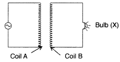
(i) Name the phenomenon involved.

(ii) If a copper sheet is inserted in the gap between the coils, explain how the brightness of the bulb would change. 

Ans.

(i) The phenomenon involved is mutual induction.

(ii) When the copper sheet is inserted, eddy currents are set up in it which opposes the passage of magnetic flux. The induced emf in coil B decreases. This decreases the brightness of the bulb.

7. Calculate the rms value of the alternating current represented in this figure. 

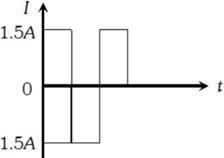
Ans. It is clear from the figure 

$i_{ms}=\sqrt{\frac{(1\cdot 5)^{2}+(1\cdot 5)^{2}+(1\cdot 5)^{3}}{3}}=1\cdot 5A$

8. If a LC circuit is considered analogous to a harmonically oscillating spring block system, which energy of the LC circuit would be analogous to potential energy and which one analogous to kinetic energy?

Ans. The energy stored in the capacitor (electrostatic energy) is analogous to potential energy and the energy stored in the inductor (magnetic energy) is analogous to kinetic energy. 

5 Important Formulas of Physics Class 12 Chapter 7 Alternating Current

Importance of Class 12 Physics Alternating Current Notes

• Revision notes help us quickly understand and remember key concepts before exams.

• They save time by focusing on essential information and skipping unnecessary details.

• These notes simplify complex topics like AC circuits, impedance, and resonance for better understanding.

• They provide practical examples that show how theoretical knowledge is used in real-life situations.

• Revision notes ensure thorough preparation by covering all important topics in a structured manner.

• They increase confidence by clearly understanding what to expect in exams.

• Accessible formats like PDFs allow for easy studying anytime and anywhere.

Tips for Learning the Physics Chapter 7 Alternating Current Class 12 PDF Notes

• Focus on understanding the basics of AC circuits, impedance, and reactance.

• Practice solving problems on resonance, power in AC circuits, and transformers.

• Memorise key formulas and their applications for quick recall during exams.

• Understand the concept of phase difference between voltage and current in AC circuits.

• Study the working principles of devices like transformers and their real-life applications.

• Solve numericals related to AC power, especially focusing on power factor and energy consumption.

Conclusion

The revision notes for Physics Chapter Alternating Current Class 12 Notes by Vedantu provide a clear and concise understanding of key concepts like AC circuits, impedance, reactance, resonance, and transformers. These notes simplify the complex topics, helping students grasp them more easily according to the current syllabus. With important formulas, diagrams, and detailed explanations, students can efficiently revise and strengthen their understanding of the chapter. These notes are a perfect tool for exam preparation, making sure students cover all the essential topics. By using notes of Alternating Current class 12 PDF, students can save time while ensuring thorough revision, enabling better performance in their exams. Download the notes today for easy learning!

Related Study Materials for Class 12 Physics Chapter 7 Alternating Current

Chapter-wise Links for Class 12 Physics Notes PDF FREE Download

Related Study Materials Links for Class 12 Physics

Along with this, students can also download additional study materials provided by Vedantu for Physics Class 12–