Theory of Consumer Behaviour Class 12 Notes CBSE Micro Economics Chapter 2 (Free PDF Download)

Consumer Behaviour: 

The study of how individual customers, groups, or organisations select, buy, use, and dispose of the ideas, goods, and services to meet their needs and wants is known as consumer behaviour. 

It refers to the consumer's actions in the marketplace and the motivations behind those actions.

Utility: 

The capacity of a commodity to meet a need is its utility. The more the utility obtained from an item, the greater the need for it or the stronger the desire to have it. Utility is a subjective concept. The same product can provide various levels of utility to different people. A consumer's desire for an item is usually determined by the utility (or satisfaction) he obtains from it.

Types of Utility

1. Cardinal Utility Analysis: This analysis suggests that utility may be stated numerically. It describes how the level of pleasure following the consumption of any goods or services can be graded in terms of countable numbers.

There can be two measures of utility, such as:

• Total Utility (TU): The total satisfaction derived from the consumption of a given quantity of a commodity at a given time is known as total utility. To put it another way, it is the total of marginal utility.

$\mathrm{TU}=\sum\mathrm{MU}\;\\\mathrm{OR}\\\mathrm{TU}\;=\;{\mathrm{MU}}_1+{\mathrm{MU}}_2+{\mathrm{MU}}_3+...+{\mathrm{MU}}_{\mathrm n}$

• Marginal Utility (MU): The marginal utility is the change in overall utility caused by the consumption of an additional unit of the commodity. To put it another way, it's the value gained from each additional unit.

${\mathrm{MU}}_{\mathrm n}={\mathrm{TU}}_{\mathrm n}-{\mathrm{TU}}_{\mathrm n-1}$

2. Ordinal Utility Analysis: It explains that the level of satisfaction following the consumption of any goods or services cannot be quantified. These items, on the other hand, can be placed in order of preference. The utility of a product is determined by its level of satisfaction. It is more realistic and logical. Indifference curve is a part of ordinal utility analysis.

Relationship Between TU and MU:

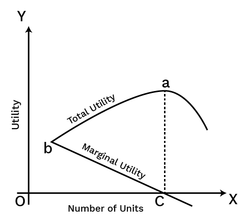
• As long as the MU is positive, the TU rises in proportion to the increase in commodity consumption. 

• TU grows/increases at a slower rate when MU from each succeeding unit starts decreasing.

• The MU becomes zero when the TU achieves its maximum value. TU stops expanding at this point, which is referred to as the point of safety. (Point c, where MU=0, and and point a where TU is maximum)

• When consumption exceeds the point of satisfaction, the MU turns negative and the TU begins to decline. (Situation after point c and a in the diagram).

Law of Diminishing Marginal Utility:

According to the law of diminishing marginal utility, as a consumer consumes more units of a commodity, the marginal benefit received from each succeeding unit declines. 

The law of demand is founded on this principle, as the concept of reduced pricing is related to the Law of Diminishing Marginal Utility. 

Consumers are prepared to spend lesser monetary amounts for more of a product as its utility falls with increased consumption.

Assumptions for this law:

• Only standard units are consumed of a commodity.

• Continuous consumption of the commodity takes place.

Table

In the table we can see that, 

• TU keeps on increasing at decreasing rate and MU is falling.

• When TU is maximum, that is 28 at 5th unit, MU becomes 0.

• After this point, MU becomes negative, as TU starts falling. 

• TU will increase only upto the situation when MU is positive, once Mu turns negative, TU starts falling.

Indifference Curve: 

• An indifference curve is a graphical representation which shows all of the product combinations that gives the same level of satisfaction to the consumer. 

• Since all of the combinations provide the same level of satisfaction, the consumer favours them all equally. As a result, the indifference curve got its name.

• A simple two-dimensional graph is used for standard indifference curve analysis. 

• Each axis represents a different form of economic good. The customer along the indifference curve is unconcerned with any of the combinations of commodities indicated by points on the curve since all of the combinations of products on an indifference curve deliver the same degree of utility to the consumer.

Table

Diagram

Explanation

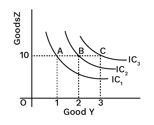
In the diagram we can see that IC3  is the highest indifference curve, as here, there are 10 units of Good Z, and 3 units of Good Y. Hence point C depicts the highest level of satisfaction.

Slope of IC: Marginal Rate of Substitution (MRS): 

The rate at which a consumer substitutes one good for another as long as the latter good is providing equal satisfaction is known as the marginal rate of substitution.

The marginal rate of substitution is the slope of the indifference curve. It is because of the MRS diminishing, that the indifference curve is convex in nature. As with increase in quantity of one good, the consumer forgoes less and less of the ther good.

$\mathrm{MRS}=\frac{\mathrm{Loss}\;\mathrm{of}\;\mathrm{Good}\;\mathrm Y}{\mathrm{Gain}\;\mathrm{of}\;\mathrm{Good}\;\mathrm X}\\\mathrm{or}\\-\frac{\triangle\mathrm Y}{\triangle\mathrm X}$

Characteristics of the Indifference Curve:

• Downward slope: Indifference curves have a downward slope i.e., slopes downward from left to right.

• Diminishing MRS: To the point of origin, indifference curves are convex. It's because the marginal rate of substitution is decreasing.

• IC’s never intersect: The curves of indifference never meet or intersect. Two points on two different ICs can't possibly provide the same level of satisfaction.

• Higher Indifference curve: A higher level of satisfaction is represented by a higher indifference curve.

• IC never touch x-axis or y-axis: An indifference curve never touches any of the axis because if it touches any one axis, that would mean the consumption of other good is zero. And, this is not possible, as IC focus on the consumption of two goods.

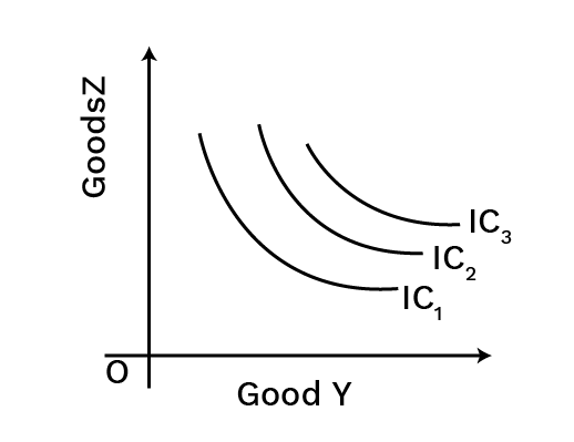
Indifference Map: 

A set of Indifference Curves constitutes an Indifference Map. It provides a comprehensive picture of a consumer's preferences. 

The diagram below depicts an indifference map made up of three curves:

Consumer Budget

• A budget limitation refers to the many combinations of goods and services that a consumer can purchase based on current prices and income. 

• The term "consumer budget" refers to the consumer's real money or purchasing power, which he can use to purchase quantitative bundles of two items at a set price. It means that a consumer can only buy goods in combination (bundles) that cost less than or equal to his income.

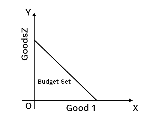
Budget Set: 

• A budget set is a quantitative collection of bundles that a consumer can buy with his current income at current market prices. 

• The budget set of a consumer is the collection of all the bundles that the consumer can purchase with his or her income at current market prices. 

• A consumer's budget set is essentially a collection of all bundles of goods and services that a consumer can purchase with available funds.

$ \Rightarrow {\mathrm p}_1{\mathrm x}_1+\;{\mathrm p}_2{\mathrm x}_2\leq\mathrm M $

Budget Line: 

The budget line is a graphical representation of all the bundles that cost the same as the consumer's income. The budget line depicts two different combinations of goods that a consumer can buy based on his or her income and commodity prices.

${\mathrm P}_{\mathrm X}{\mathrm Q}_{\mathrm X}+{\mathrm P}_{\mathrm Y}{\mathrm Q}_{\mathrm Y}=\mathrm S$

Here,

${\mathrm P}_{\mathrm X}$ = Price of commodity X

${\mathrm Q}_{\mathrm X}$ = Quantity of commodity X

${\mathrm P}_{\mathrm Y}$ = Price of commodity Y

${\mathrm Q}_{\mathrm Y}$ = Quantity of commodity Y

S = Consumer Income

Attainable and Non Attainable Combinations

Any point within the area budget line is an attainable combination that a consumer can buy given his income and price of goods. Any point outside the area is a non-attainable combination, which the consumer cannot afford to buy.

Budget Constraint: 

The budget constraint includes all the different combinations of goods or products that a person can afford based on the cost of goods and consumer income.

For example:

Q1 is the quantity of Good 1, 

Q2 is the quantity of Good 2, 

P1 is the price of Good 1, 

P2 is the price of Good 2. 

P1q1 = Total amount spent on Good 1. 

P2q2 = Total amount spent on Good 2. 

As a result, the budget line equation will be p1q1 + p2q2 = X. The budget line is always slanted downward, so consumers can only raise their consumption of Good 1 by decreasing their consumption of Good 2. 

If customers want to buy one more unit of Item 1, they may only do so if they are willing to give up some quantity of another good. Consumers have a restricted budget. They must decide whether to spend money on Good 1 or Good 2.

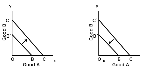
Changes or Shifts in Budget Line: 

• Due to changes in the consumer's income and the price of goods, there may be a parallel shift such as leftwards or rightwards shift. 

• A rise in consumer income shifts the budget line to the right, and vice versa.

• There will be a rotation in the budget line if the price of one good changes. When prices fall, purchasing power rises, causing outward rotation, and vice versa.

• In Figure A, when the consumer income increases, budget line shifts from BB’ to CC’, as now the consumer can afford more of both the goods, keeping price constant.

• In the figure B, when the consumer income increases, budget line shifts from CC’ to BB’, as now the consumer can afford less of both the goods, keeping price constant. 

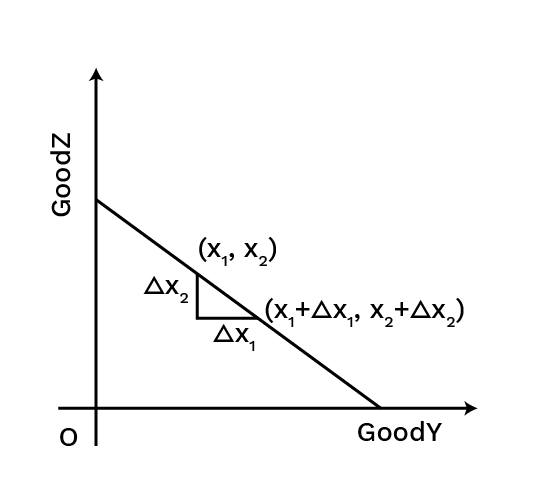
Derivation of the Slope of the Budget Line: 

The budget line's slope indicates how much change in good 2 is necessary per unit of change in good 1 along the budget line. 

Let us now calculate the slope of the budget line as follows:

On the budget line, take two points.

Say, $\left({\mathrm x}_1,{\mathrm x}_2\right) and \left({\mathrm x}_1+\triangle{\mathrm x}_1,{\mathrm x}_2+\triangle{\mathrm x}_2\right)$

${\mathrm p}_1{\mathrm x}_1+{\mathrm p}_2{\mathrm x}_2=\mathrm M\;.....\;\left(1\right)\\{\mathrm p}_1\left({\mathrm x}_1+\triangle{\mathrm x}_1\right)+{\mathrm p}_2\left({\mathrm x}_2+\triangle{\mathrm x}_2\right)=\mathrm M\;.....\;\left(2\right)$

Subtracting (1) from (2), we get

${\mathrm p}_1\triangle{\mathrm x}_1+{\mathrm p}_2\triangle{\mathrm x}_2=0\\\frac{\triangle{\mathrm x}_2}{\triangle{\mathrm x}_1}=-\frac{{\mathrm p}_1}{{\mathrm p}_2}$

Changes in Budget Set: 

• The available bundles are determined by the prices of the two commodities and the customer's earnings. 

• The set of available bundles is likely to change when the price of either of the commodities or the customer's earnings changes.

Assume the customer's earnings increase from N to N′ while the prices of the two(2) commodities stay unchanged. The customer will be able to purchase all bundles with his new earnings $\left({\mathrm x}_1,{\mathrm x}_2\right)$ such as ${\mathrm p}_1{\mathrm x}_1+{\mathrm p}_2{\mathrm x}_2\leq\mathrm N'$

The budget line's equation is now:

 ${\mathrm p}_1{\mathrm x}_1+{\mathrm p}_2{\mathrm x}_2=\mathrm N'$

The above equation can also be written as ${\mathrm x}_2=\frac{{\mathrm N}_1}{{\mathrm p}_2}-\frac{{\mathrm p}_1}{{\mathrm p}_2}\;{\mathrm x}_1$

It is worth noting that the slope of the new budget line is identical  as it was before the customer's earnings changed.

Consumer’s Optimum Choice: 

• The Indifference Curve and Budget Line can be used to explain the condition for a consumer's optimal choice of two goods. 

• The satisfaction curve is represented by the indifference curve, whereas the budget line is represented by the budget line. 

• Given a budget constraint, a consumer would want to get the most out of two goods. As a result, he will strive for the highest IC possible while staying within his financial constraints. 

• A consumer equilibrium can occur when:

• IC is convex to the point of equilibrium.

• Slope of IC = Budget Line Slope

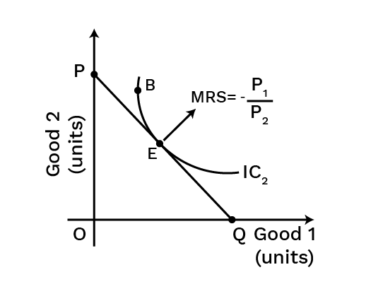
In the diagram, where the IC curve is tangent to the budget line, that is point E is the optimal choice, and also a point of consumer equilibrium. This is the point where the slope of both, the indifference curve and budget line are equal to each other.

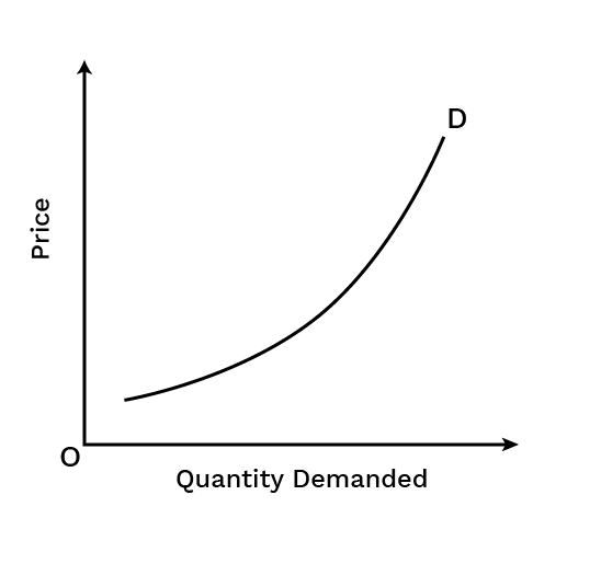
Demand: 

The quantity that a consumer is able and willing to purchase at a specific price and within a specific time frame.

Demand Function: 

The demand function represents the functional relationship taking place between a commodity's quantity demanded and its various determinants.

Dx= f(Px, PR, Y, T, E)

Here, 

Dx= Quantity Demand 

f= Functional Relationship

Px= Own price of good

PR= Related price of good

Y = Income

T= Taste and Preferences

E= Expectations

Factors affecting Demand:

• Product Price: The price of a commodity has an inverse (negative) relationship with the amount of that commodity that buyers are willing and able to buy. Consumers prefer to buy more of a low-priced commodity and less of a high-priced commodity. The inverse relationship between price and the amount of money people are willing and able to spend is known as The Law of Demand.

• Consumer’s Income: The impact that pay has on the measure of a product that purchasers are willing and ready to purchase relies upon the sort of good we're discussing. 

• Normal Goods: For most products, there is a positive (direct) connection between a consumer's income and the measure of the decency that one is willing and ready to purchase. At the end of the day, for these merchandise when income grows the interest for the product will increase; when the income falls, the interest for the product will diminish. These are referred to as normal goods. 

• Inferior Goods: However, for other commodities, a change in income has the opposite impact. An inferior good is one whose demand decreases as wealth grows. In other words, customer demand for inferior items is inversely connected to income. In economics, inferior suggests that there is an inverse association between one's income and the interest or demand for that commodity. 

Furthermore, whether a good is normal or inferior may differ from one individual to the next. For you, a commodity could be normal good, but for someone else, it might be inferior.

• Price of Related Goods: Assuming that the commodity price remains constant, there are two categories of linked products that impact demand for the commodity. 

• Complementary Goods: Complementary goods are linked products that are consumed together because their utility is reduced if consumed alone. As a result, if demand for one of the two products rises, demand for the other rises as well, even though the price of this commodity stays unchanged, and vice versa.

• Substitute Goods: Substitute goods are commodities that are diametrically opposed to one another. As a result, if demand for one of the two products increases, demand for the other product falls even though the price of this product stays constant, and vice versa.

• Taste and preferences of consumer: A favourable change in tastes and preferences of consumer leads to increase in demand, while the opposite happens when there is a negative change in taste and preference of consumers.

• Expectation: If the consumer expects that the availability of a good in the future is going to fall, his present demand of that good would increase, and vice versa, keeping the price constant.

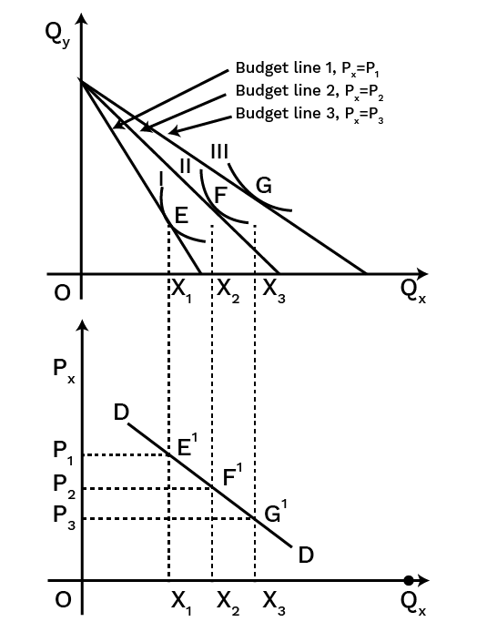
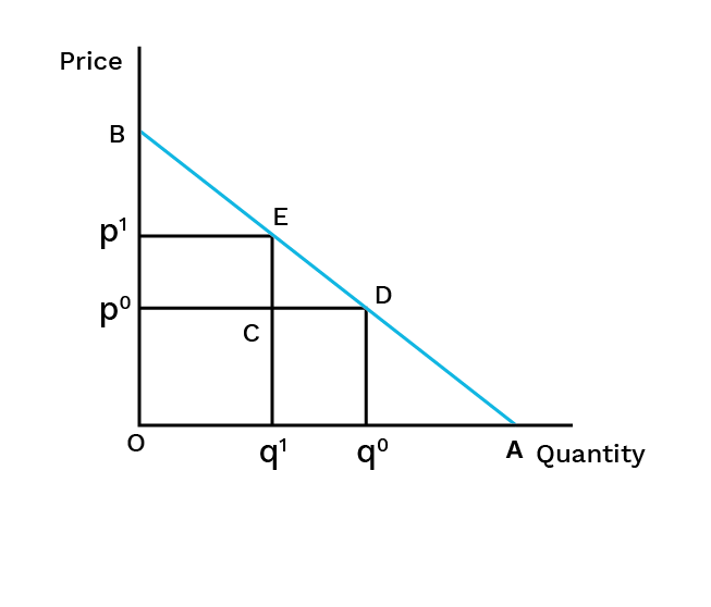
Derivation of Demand Curve: 

According to the IC analysis, a buyer maximises his utility by selecting a package of two commodities that is also within his budget. This will be used to calculate a commodity's demand curve. 

• Consider the following two items: X and Y. Let the two items' prices be ${\mathrm P}_{\mathrm x}$ and ${\mathrm P}_{\mathrm y}$ , and the monetary income will be ‘M.’ 

• At the point where the consumer's budget line intersects the indifference curve, he can maximise his utility. In the diagram, this would be point ‘E.' ${\mathrm X}_1$ is the amount of X consumed.

• We now modify the price level of good X while maintaining the price of good Y and the amount of money income constant. 

• Allow ${\mathrm P}_{\mathrm x}$ to fall. With the same amount of money, the consumer's real purchasing power has increased. 

• Because ‘M’ remains constant, the greatest amount of good X he can buy grows as ${\mathrm P}_{\mathrm x}$ declines. 

• As a result, the budget line's horizontal intercept changes (shifts to the right). However, the vertical intercept remains unchanged since ‘M’ and ${\mathrm P}_{\mathrm y}$ remain constant. 

• As a result, as ${\mathrm P}_{\mathrm x}$ declines, the budget line must pivot away from the origin along the horizontal axis.

Law of Demand

The effects of price changes on the amount desired of an item are described in the form of a law known as the law of demand.

It asserts that when the price of an item decreases, the amount required rises, and when the price of a commodity rises, the quantity demanded declines. In other words, if everything else remains constant, the price of a commodity and its quantity requested have an inverse relationship.

Exception to the Law of Demand 

In some circumstances, when the price rises, the amount demanded ascents as well (and vice versa). The exceptions are:

1. Articles of Distinction: When the good in consideration is one of status. As the price grows, so must the amount requested in order to maintain the prestige value. For example, antique pieces, precious jewels etc. Also, the demand for these goods is only because of their high prices.

2. Goods of Necessity: When the good is of basic necessity, demand rises even if the price rises since the good is a requirement.

3. Giffen Good: When the good under consideration is a Giffen good.

Types of Goods

• Normal Goods: A normal good is one whose demand rises in response to an increase in the consumer's income or pay.

• Inferior Goods: Inferior goods are those whose demand declines as the consumer's income rises. As a result, as consumer affordability rises, so does the demand for lower-quality goods.

• Giffen Goods: It is a low-income, non-luxury item that contradicts conventional economic and consumer demand theories. When the price rises, demand for Giffen items rises, and when the price falls, demand for Giffen goods reduces. 

• Substitutes Goods:  These are identical goods that can be utilised interchangeably to some extent. For example, tea and coffee are substitutes.

• Complementary Goods: These are items that are typically consumed together and complement one another. For example car and petrol.

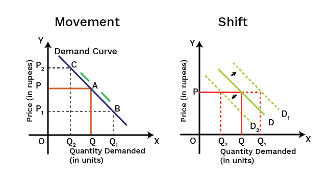
Shift in demand curve: 

• A shift in the demand curve indicates changes in demand at each potential price as a result of changes in one or more non-price factors such as the price of comparable commodities, income, taste & preferences, and consumer expectations. 

• The equilibrium point shifts whenever the demand curve shifts. 

• The demand curve shifts to one of two directions: 

• rightward shift or 

• leftward shift. 

• The price does not change, factors other than price cause a shift in demand.

Movement along the Demand Curve:

• The movement of the demand curve indicates the variation in both the price and the quantity demanded from one position to the other. 

• When the quantity demanded changes owing to a change in the price of the product or service, the demand curve moves. 

• The movement along the curve can occur in either of two directions: 

• upward movement or 

• downward movement.

Difference - Movements along the Demand Curve and Shifts in the Demand Curve:

The following points are noteworthy in terms of the distinction between movement and shift in the demand curve:

Diagrammatic Representation of Movements along the Demand Curve and Shifts in the Demand Curve

Market Demand:

• The total quantity of an item sought in the market by all consumers at various prices at a given moment is known as market demand.

Elasticity of Demand: 

• The price elasticity of demand measures how a change in price affects the demand for a product among its consumers. 

• It is calculated by dividing the percentage change in a product's required quantity by the percentage change in the product's cost. This is also called percentage method of elasticity of demand,

${\mathrm e}_{\mathrm d}\;=\frac{\;\mathrm{percentage}\;\mathrm{change}\;\mathrm{in}\;\mathrm{demand}\;\mathrm{for}\;\mathrm{the}\;\mathrm{good}}{\mathrm{percentage}\;\mathrm{change}\;\mathrm{in}\;\mathrm{the}\;\mathrm{price}\;\mathrm{of}\;\mathrm{the}\;\mathrm{good}}\\{\mathrm e}_{\mathrm d}=\frac{\triangle\mathrm Q}{\triangle\mathrm P}\times\frac{\mathrm P}{\mathrm Q}$

Here,

${\mathrm e}_{\mathrm d}$ = Elasticity of demand

$\triangle\mathrm Q$ = Change in quantity

$\triangle\mathrm P$ = Change in price

P = Initial price

Q = Initial Quantity

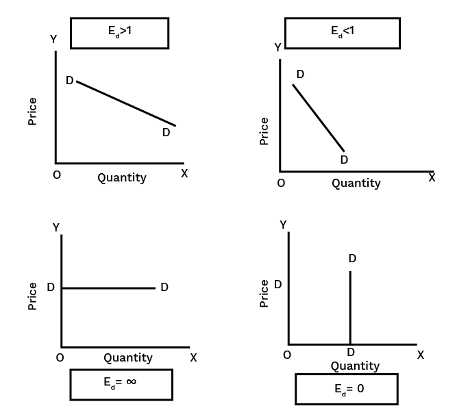
Situations of Elasticity of Demand:

1. Ed= 1: Also, called unitary elastic demand, or rectangular hyperbola. When change in demand and change in price is in the same proportion. A 10% increase in price leads to a 10% decrease in demand.

2. Ed> 1: When change in demand is greater than the change in price. A 10% fall in price leads to a 30% increase in demand.

3. Ed< 1: When change in demand is less than the change in price. A 30% decrease in price leads to a 10% increase in demand.

4. Ed= ∞: It is also called perfectly elastic demand, as here the demand is infinity at the current price. Any change in price would cause demand to fall to zero.

5. Ed= 0: It is called perfectly inelastic demand, as here, irrespective of price change, demand remains constant.

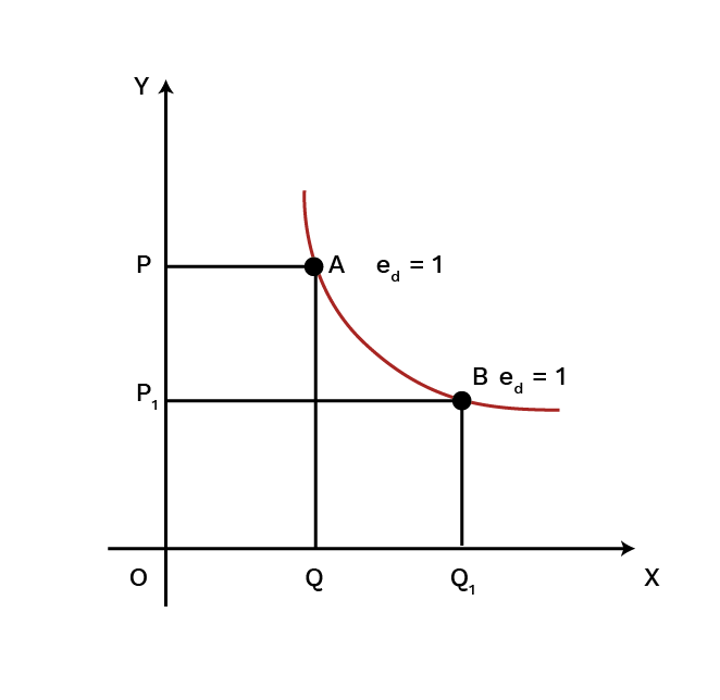
Rectangular Hyperbola (ed=1) : 

A rectangular hyperbola is a curve with equal rectangular areas on all sides. When the elasticity of demand equals one (ed = 1) at all points along the demand curve, the demand curve is indeed a rectangular hyperbola. As given in the figure beneath it is a  downward-sloping curve.

Geometric Method of Elasticity of Demand: 

Elasticity of demand is measured at any location by dividing the length of the lower segment of the demand curve by the length of the upper segment of the demand curve at that point. At the midpoint of any linear demand curve, the value of ed is unity.

A linear demand curve's elasticity may be simply assessed graphically. The elasticity of demand at each point on a straight line demand curve is determined by the ratio between the demand curve's lower and upper segments at that position.

${\mathrm e}_{\mathrm d}=\frac{\mathrm{DA}}{\mathrm{DB}}$

Total Expenditure Method of Elasticity of demand: 

• It calculates the price elasticity of demand based on the change in total expenditure(Product of Price and quantity) incurred by a household on the commodity as a result of a price change. 

• The price of a commodity and its demand are inversely linked. 

• The responsiveness of the demand for the commodity to price changes determines whether expenditure on the good increases or decreases as a result of a rise in its price.

Relationship between Total Expenditure and Price of Elasticity of Demand:

• $\;{\mathrm E}_{\mathrm d}=1$ When total spending (price X quantity) remains constant despite a rise or reduction in the price of a good.

• ${\mathrm E}_{\mathrm d}>1$ When prices fall, total expenditure rises, and when prices rise, total expenditure falls.

• ${\mathrm E}_{\mathrm d}<1$ When total expenditure falls as a result of a price decrease and total expenditure rises as a result of a price increase.

Factors that influence price elasticity of demand:

• Availability of close substitutes: Demand for a commodity with many equivalents is typically more elastic than demand for goods with no replacements. Coca-Cola, Pepsi, Limca, and other similar beverages are suitable replacements. Even a minor increase in the price of coke will entice purchasers to seek alternatives. Electricity demand, on the other hand, will be less elastic because there are no close substitutes.

• Nature of the Commodity: Demand for essentials such as medicines and food grains is less elastic since we must consume them in the lowest quantity required, regardless of price. In any case, elasticity for comfort and extravagances like refrigerators, air conditioners and so on is more flexible on the grounds that their utilization might be delayed in the future if their cost rises.

• Price level: Demand for a higher-priced commodity such as air conditioners or automobiles is often more elastic than demand for a lower-priced commodity such as match box or pencils.

• Income level: Higher income groups have less elastic demand for commodities than lower income groups. For example, if the price of a commodity rises, a wealthy consumer is unlikely to cut his demand, whereas a poor buyer may.

Theory of Consumer Behaviour Class 12 PDF

These CBSE Economics Class 12 Chapter 2 notes are available in PDF format, making it easy to download and use these notes on the go. Whether you are travelling or waiting for a doctor’s appointment, once you download these notes, you need to go through them at your comfort and pace. You can refer to them even before an examination, be it a school or competitive exam. Students can also print these Microeconomics Class 12 Chapter 2 notes in hardcopy, making it easy to revise through them.

Theory of Consumer Behaviour Class 12 Revision Notes

Our revision notes cover Microeconomics Class 12 Chapter 2 in great detail.

• The consumer is an agent who consumes the final good or the services.

• The utility is the wants or the satisfying power of the commodity. The total utility is the satiation that gets derived when one consumes the given amount of commodity at one given time. The total utility is the sum of the total marginal utility.

• Marginal utility is the change that occurs in the total utility that results from the consumption of the additional commodity unit. It is the added utility that gets derived when one consumes an additional unit.

• The law of diminishing marginal utility is when the consumer consumes more of the commodity units; the marginal utility starts to decrease. This is the law of demand.

• Consumers bundle is the quantitative combination of two goods purchased by the consumer from his income.

• The Law of Equi-marginal utility is where a consumer spends his income on various commodities; then he attains an equilibrium, which is the maximum satisfaction at that point. This is calculated as the ratio of the marginal utility and the prices of various commodities that are equal. This, in turn, equals the marginal utility of money.

• The budget set is the quantitative combination of the bundle that the consumer can purchase from his income at the market's prevailing prices.

• Consumer Budget states the consumer's real purchasing power is from which he is capable of purchasing some quantitative bundles of two goods at one given price.

• Budget Line is the graphical representation of all the bundles that cost the amount equal to the consumer's money income. This helps to draw the budget line.

Monotonic Preferences

The preferences of the consumer are known as monotonic preferences. This is where one bundle has more than the other of one good and not less of the other good in between two bundles. This offers a high level of satisfaction.

Change in Budget Line

It is possible that there can be a parallel shift in the budget line. This could be towards the left or the right. The change happens because of the change in the consumer's income and a change in the goods' prices. When there is a rise in consumer income, it shifts the budget line towards the right. When there is a drop in the consumer's income, it shifts the budget line to the left. If there is a change in the price of one of the goods, this causes the budget line to rotate. The fall in the price causes outward radiation, which happens because there is a rise in the purchasing power of money.