


Production and Costs Class 12 Extra Questions and Answers Free PDF Download
Free PDF download of Important Questions with Answers for CBSE Class 12 Micro Economics Chapter 3 - Production and Costs prepared by expert Economics teachers from the latest edition of CBSE(NCERT) books. Register online for Online tuition on Vedantu.com to score more marks in the CBSE board examination.
 Table of Content
Multiple Choice and Very Short Answer Questions - 1 Mark
1. What is meant by production?
Ans: Production refers to the translation of input into output via a specific process.
2. What will be the MP when TP is maximum?
Ans: When the Total Product (TP) is at its maximum, the Marginal Product (MP) will be zero.
3. When there are diminishing returns to a factor, total product always decreases.
Ans: False, because TPP grows at a lower rate when a factor's returns diminish.
4. TPP increases only when MPP increases.
Ans: True, TPP increases as MPP falls but remains positive.
5. Increase in TPP always indicates that there are increasing returns to a factor.
Ans: True, TPP grows even while the returns to a factor are diminishing.
6. When there are diminishing returns to a factor, marginal and total product always fall.
Ans: False; only the MPP is in jeopardy, not the TPP. TPP increases at a decreasing pace when there are diminishing returns to a factor.
7. Calculate MP for the following.
Ans:
8. Why does the AFC curve never touch the “x‟ axis though it lies very close to the x axis?
Ans: TFC can never be equal to zero.
9. Why are AVC and AFC usually lower than AC?
Ans: Since AC is the sum of AVC and AFC, it is always greater than AVC and AFC.
10. Why does the TVC curve start from the origin?
Ans: At zero output level, TVC is zero.
11. When TVC is zero at zero level of output, what happens to TFC or Why TFC is not zero at zero level of output?
Ans: Even if output is zero, fixed costs must be incurred.
12. Production function shows technical relationship between physical inputs and output of a commodity
1. Technological relationship between inputs and cost
2. Economic relationship between inputs and output
3. Technological relationship between inputs and output
4. Technological relationship between inputs and price
Ans: (3) Technological relationship between inputs and output
13. In the short run TPP changes with the change in which of the following factors
1) Economic cost
2) Fixed factors
3) All the factors
4) Variable factors
Ans: (4) Variable factors
14. How is TPP derived from MPP?
1) Cumulative addition
2) Cumulative subtraction
3) Cumulative product
4) Cumulative division
Ans: (1) Cumulative addition
15. The general shape of TPP in the short run is
1) Inverse U shaped
2) U shaped
3) Hyperbola
4) V- shaped
Ans: (1) Inverse U shaped
Short Answer Question - 3 or 4 Marks
16. What are Returns to a Factor? What do you mean by the Law of Diminishing Returns?
Ans: Returns to a Component is used to explain the behavior of physical output by allowing only one factor to vary while keeping all other factors constant. This is a short-term idea. According to the rule of diminishing returns to a factor, as the variable factor is allowed to vary (grow) while all other factors remain constant, the Marginal Product initially climbs, reaches its maximum, then drops and even becomes negative.
17. What is the change in quantity demanded?
Ans: It is often referred to as movement along a demand curve. The quantity of a commodity fluctuates due to a change in its own price due to the shift in the supply curve. There are two types of changes in demand quantity:
(a) expansion in demand
(b) contraction in demand.
18. What is the change in demand?
Ans: Demand Variation: - It is also known as a change in the demand curve. When the quantity of a commodity changes as a result of a change in a factor other than price. It comes in two varieties.
a) Increase in demand
b) Decrease in demand
19. Define cost concept. What are the different types of costs?
Ans: The cost of production refers to the money spent on various inputs. The different types of costs are explained below:
i. Money Cost: The total amount of money spent by a company to produce a commodity.
ii. Explicit Cost and Implicit Cost: Explicit Cost is the actual payment made to outsiders. The cost of self-supplied factors is included in the implicit cost.
iii. Real Cost: All of the suffering, sacrifices, and discomforts associated with producing factor services to produce commodities.
iv. Opportunity Expense: This is the cost of foregoing the next best alternative.
v. Short Run Cost:
I. Fixed Cost: - Cost of fixed factors.
II. Variable Cost: - Cost of variables.
Relationship between AC, MC, and AVC:
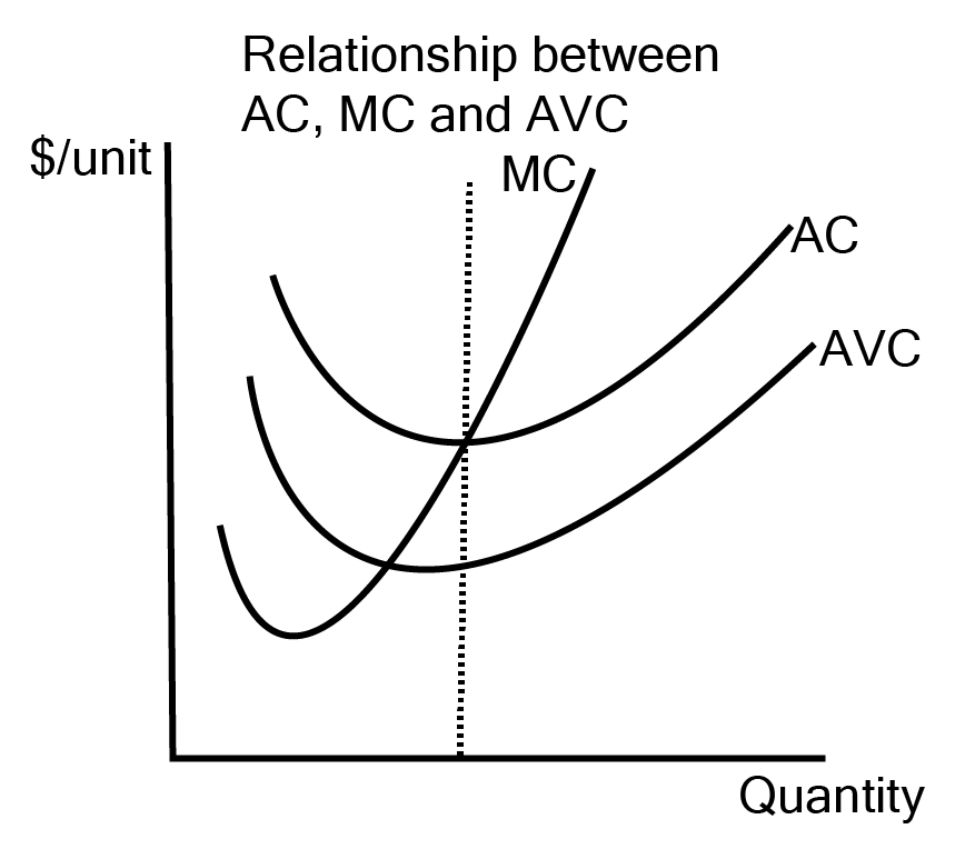
• If MC is less than AC, AC tends to fall.
• When MC equals AC, AC is the smallest.
• When MC is greater than AC, AC tends to rise.
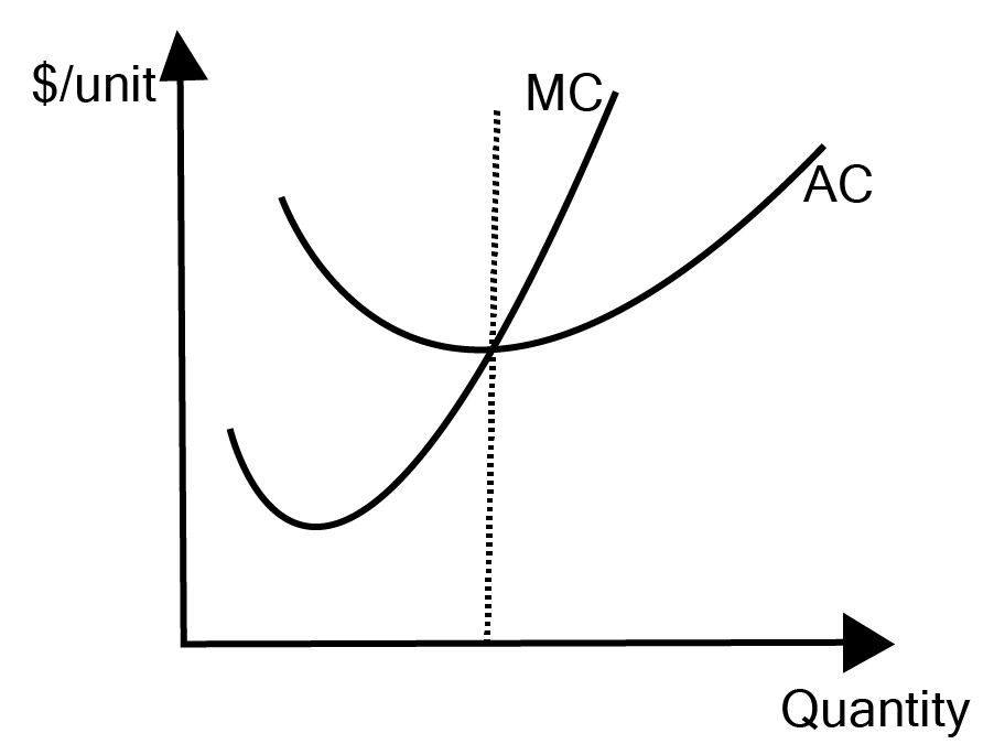
20. Explain the relation between AC and MC with the help of a diagram.
Ans: The following figure depicts the relationship between AC and MC:
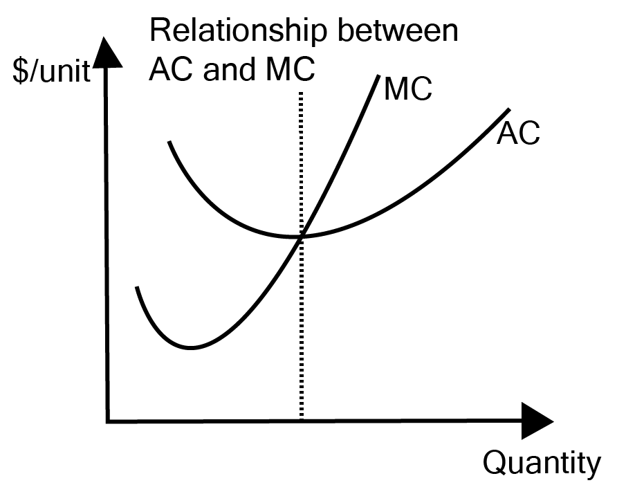
Observations:
(i) When AC falls, MC falls quicker than AC. As a result, the MC curve remains below the AC curve. implying that AC is greater than MC In the graph, the AC curve falls until point A, while the MC curve remains lower than the AC curve.
(ii) As AC rises, MC rises faster than AC. As a result, the MC curve is higher than the AC curve. Inferring that AC MC. In the diagram, AC begins to rise from point A, and beyond A, MC exceeds AC.
(iii) The MC curve cuts the AC curve at its lowest point. When the average curve is the smallest, MC = AC. In the illustration, the MC curve intersects the AC curve at its lowest or minimum point A.
Long Answer Questions 6 Marks
21. Explain the relation between Marginal Cost and Average Variable Cost with the help of a diagram.
Ans: One of the various cost relationships is the one that exists between marginal cost and average variable cost. When the marginal cost is smaller than the average variable cost, the average variable cost falls. On the contrary, when marginal cost exceeds average variable cost, average variable cost rises. This may also imply that average variable cost takes on a U-shape in some circumstances, albeit this is not guaranteed because neither average variable cost nor marginal cost have a fixed cost component. In business, both fixed and variable expenses are utilized to calculate production costs. The change in production expenses for each extra item is measured by marginal costs. The materials required to manufacture or make each product are reflected in variable costs. As a result, variable expenses have a direct impact on the marginal cost.
Let’s take an example, Mary, who owns a bakery and is thinking about expanding her existing range beyond cakes. Sandwiches will be another new item. However, she will need to consider both the variable and marginal expenses to determine whether it is worthwhile. She should compute the average cost of the additional ingredients and labor required to produce the sandwiches. The marginal cost will then be calculated using the variable and constant costs. If the marginal cost of a sandwich is too high to generate a profit, she will not bother adding it.
22. Explain the determinants of supply?
Ans: The quantity of a good available for sale at a given price at a given time is referred to as supply. A desired flow is supply. It assesses how much a corporation is willing to sell rather than how much it actually sells. Supply may outnumber or fall short of demand. In a given year, supply equals total output plus or minus inventories of the commodity.
The supply function can be written as:
Sx = f(Px, Pa… Pc, PL… PO, T, Cr, St, O, G)
Here, Px is the price of the good x, Pa... Pc is equal to the prices of related items, PL... PO is the prices of inputs, T is time, St is the state of technology, O is the firm aims, and G is the taxes, subsidies, and regulation.
The determinants of the supply are shown below:
i. Price of product
ii. Price of related goods
iii. Consumer’s income
iv. Consumers tastes and preferences
v. Advertisement expenditure
vi. Consumer’s expectations
vii. Demonstration effect
viii Population of the country
ix. Distribution of national income
Some of the determinants are discussed below:
i. Production costs - Because the purpose of most private companies is profit maximization. Higher production costs reduce profit, limiting supply. Factors influencing manufacturing costs include input prices, wage rates, government regulations and taxes, and so on.
ii. Technology - Technological advancements assist cut production costs and enhance profit, resulting in increased supply.
iii. Number of sellers - The presence of more sellers in the market increases market supply.
iv. Future price expectations - If producers anticipate that future prices will be higher, they will want to hang onto their stocks and offer the items to consumers in the future, allowing them to collect the higher price.
23. State the behaviour of Marginal product is the Law of Variable Proportions. Explain the causes of this behaviour.
Ans: According to the law of variable proportion, the marginal product of the factor input initially grows with the degree of employment. However, once it hits a certain level of employment, it begins to plummet.
The picture below explains this law very well:
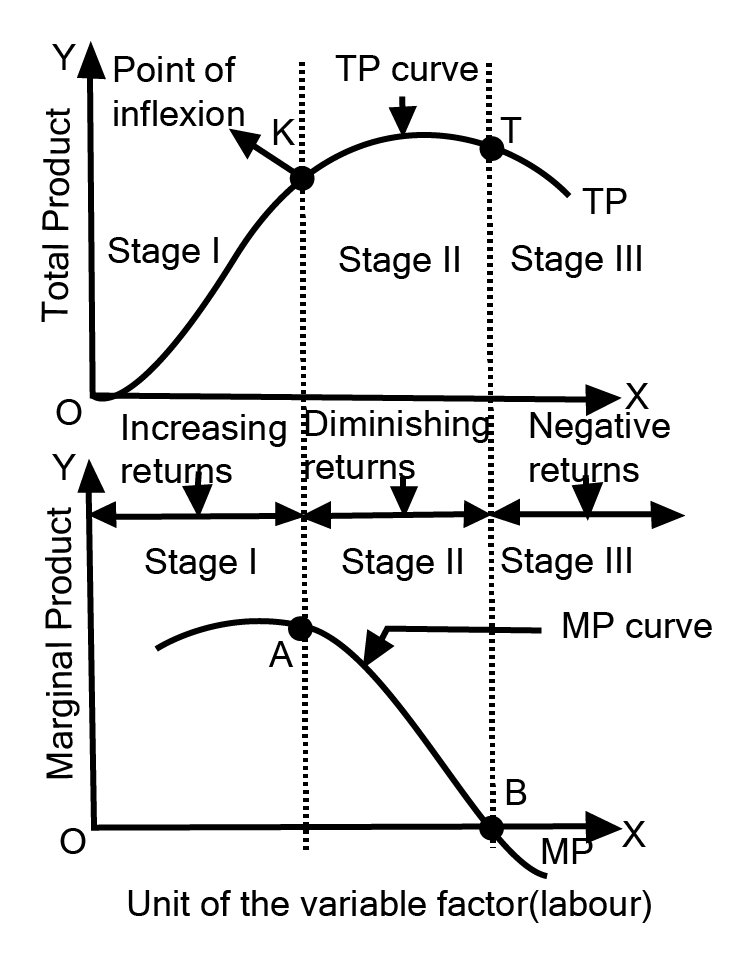
AP = TP/Q MPnth = TPn - TPn-1
We can make the following observations based on the graphic and table above:
(i) MP rises until the third unit of labor is employed. In this case, TP rises at an increasing rate and hence, this is known as the condition of increasing retirements.
(ii) With the use of the fourth unit of labor, MP begins to decrease and TP only increases at a decreasing rate. This is known as the condition of diminishing returns.
(iii) When the MP is reduced to zero, the total product is maximized.
(iv) When the marginal product is negative, total products begin to fall. The law of variable proportion is based on diminishing returns to the marginal factor, and the causes are flawed factor sustainability, poor factor coordination, and so on.
Important Study Material Links for Class 12 Microeconomics Chapter 3
CBSE Class 12 Economics Important Questions Textbooks
Chapter-wise Links for Microeconomics Class 12 Questions
Related Study Materials Links for Class 12 Microeconomics
Along with this, students can also download additional study materials provided by Vedantu for Microeconomics Class 12–

FAQs on Important Questions For Class 12 Micro Economics Chapter 3 Production and Costs - 2026-27
1. What are the most expected 5-mark questions for CBSE Class 12 Micro Economics Chapter 3 - Production and Costs in the 2026–27 board exam?
For the 2026–27 boards, important 5-mark questions may include:
- Explaining the Law of Variable Proportions with a diagram and stages
- Describing the relationship between Average Cost (AC) and Marginal Cost (MC) using a labeled curve
- Discussing the types of production costs with real-life examples
2. Which short answer questions from Production and Costs are important for achieving marks efficiently in CBSE exams?
Expected short answer questions (1- or 3-marks) often cover:
- Definition of Total Product (TP), Average Product (AP), and Marginal Product (MP)
- Difference between Total Variable Cost (TVC) and Total Fixed Cost (TFC)
- Shape and behavior of the Average Fixed Cost (AFC) curve
3. How should students approach HOTS (Higher Order Thinking Skills) questions from Production and Costs for maximum marks?
To excel in HOTS questions:
- Analyze scenarios using the Law of Diminishing Returns
- Interpret diagrams showing the relationship between different cost curves
- Apply opportunity cost concepts to real-life business choices
4. What marking trends and question types are observed in CBSE Class 12 board exams for Production and Costs?
Recent marking trends show repetitive focus on:
- Short run vs long run costs distinctions
- Law of Variable Proportions with stages and diagrammatic clarity
- Real-life illustrations of explicit and implicit costs
5. How can students avoid common conceptual traps when answering questions on the Law of Variable Proportions in board exams?
Avoid these traps:
- Incorrectly assuming Total Product (TP) decreases as soon as returns diminish; TP still rises but at a slower rate
- Confusing the three stages—optimal output lies in the diminishing returns (Stage II), not when MP is negative
- Mislabeling axes or curves in diagrams
6. Why does the Average Fixed Cost (AFC) curve never touch the x-axis in cost diagrams?
Average Fixed Cost (AFC) is calculated as Total Fixed Cost divided by output (AFC = TFC/Q). Since TFC is always positive, AFC approaches zero as output increases but never reaches it, resulting in a curve that never touches the x-axis. This concept is frequently tested for 1-mark clarity in CBSE exams.
7. How does understanding Marginal Cost (MC) help in decision-making for producers, as per CBSE exam expectations?
Marginal Cost (MC) shows the additional cost of producing one more unit. Producers use MC to determine the most profitable output level, set competitive pricing, and minimize losses. Board questions often test the application of MC concepts for managerial decisions and production planning.
8. What is the relationship between Average Cost (AC) and Marginal Cost (MC), and how can it be tested in board exam diagrams?
The relationship includes:
- If MC < AC, AC falls
- If MC > AC, AC rises
- MC intersects AC at AC's minimum point
9. Compare explicit and implicit costs with examples relevant to the CBSE syllabus.
Explicit costs are actual payments made to outside resources, for example, wages paid to hired workers. Implicit costs refer to the value of self-owned resources, such as the foregone salary of an entrepreneur managing their own business. Both are integral in calculating total economic cost and are key board exam topics.
10. Why is Total Variable Cost (TVC) zero at zero output, while Total Fixed Cost (TFC) remains constant?
When output is zero, no variable inputs are used, so TVC is zero. However, TFC such as rent or salaries must still be paid, regardless of output level. This distinction is frequently tested through direct 1-mark questions in CBSE board exams.
11. How can the Law of Diminishing Marginal Product influence cost curves in the short run?
As the Law of Diminishing Marginal Product sets in, Marginal Product decreases. This makes Marginal Cost (MC) rise as more variable inputs are added, causing the MC and Average Variable Cost (AVC) curves to slope upward—an important CBSE cost analysis trap area.
12. What is the importance of opportunity cost in production decision-making for board questions?
Opportunity cost represents the value of the next best alternative foregone. It is crucial for evaluating alternative production options, resource allocation, and maximizing efficiency—frequently tested in application-type CBSE questions to assess economic reasoning.
13. What are the different types of production costs as per CBSE Class 12 syllabus, and give examples?
There are several types:
- Money cost (actual expenditure on production)
- Explicit cost (paid out, e.g., wages)
- Implicit cost (unpaid, e.g., owner’s input)
- Real cost (physical efforts and sacrifices)
- Opportunity cost (next best use foregone)
- Fixed cost (rent, salaries)
- Variable cost (raw materials, power)
14. How can students best demonstrate the relationship between Average Variable Cost (AVC) and Marginal Cost (MC) in CBSE exam answers?
Board answers should state:
- If MC is below AVC, AVC falls
- If MC exceeds AVC, AVC rises
- The MC curve intersects AVC at its lowest point
15. How do technological advancements affect cost curves in the short run, as per CBSE board exam standards?
Technological improvements increase production efficiency, reducing Average Cost (AC) and Marginal Cost (MC) at each output level. This often causes the curves to shift downward. Board questions may ask for analysis or diagrammatic impact to check application of this concept.