


What Is the Role of Displacement Current in Maxwell’s Equations?
Displacement current is a fundamental concept introduced by Maxwell to address the limitations of Ampere’s law in the context of time-varying electric fields. This correction led to the formulation of Maxwell’s equations, which collectively describe the behavior of electric and magnetic fields and underpin the theory of electromagnetism. These equations are essential for understanding electromagnetic wave propagation and are a key part of the JEE Physics curriculum.
Maxwell’s Equations: The Basis of Electromagnetic Theory
Maxwell’s equations establish the mathematical relationships between electric fields, magnetic fields, charge distributions, and currents. Together, these four equations unify electrostatics and magnetostatics with time-varying electromagnetic phenomena.
Electrostatics deals with stationary charges, where electric and magnetic fields act independently. Magnetostatics considers steady currents, resulting in static magnetic fields. However, time-varying fields require a comprehensive approach provided by Maxwell’s equations. The fundamentals of electric and magnetic field behavior are also discussed in Coulomb's Law.
Mathematical Form of Maxwell’s Equations
The four Maxwell’s equations, presented in both differential and integral forms, encapsulate the following physical laws:
| Physical Law | Equation (Differential Form) |
|---|---|
| Gauss’s Law for Electricity | $\nabla \cdot \vec{E} = \dfrac{\rho}{\varepsilon_0}$ |
| Gauss’s Law for Magnetism | $\nabla \cdot \vec{B} = 0$ |
| Faraday’s Law of Induction | $\nabla \times \vec{E} = -\dfrac{\partial \vec{B}}{\partial t}$ |
| Ampere-Maxwell Law | $\nabla \times \vec{B} = \mu_0 \vec{J} + \mu_0 \varepsilon_0 \dfrac{\partial \vec{E}}{\partial t}$ |
The integral forms connect the fields to physical quantities like enclosed charge and current. These relations are central to problems on Electric Field Lines and flux calculations.
Analysis of the Ampere’s Law Limitation
Ampere’s Law in its original form works correctly for steady currents but fails for time-dependent situations such as a charging capacitor. In these cases, the current is not continuous through all regions of space, leading to a discrepancy in the predicted magnetic field.
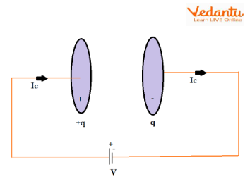
For instance, during the charging of parallel plate capacitors, there is a conduction current in the wires, but no actual current through the space between the plates. However, a changing electric field exists in this region, as further explained in Electrostatic Potential and Capacitance.
Origin and Definition of Displacement Current
To resolve the limitation of Ampere’s Law, Maxwell introduced the concept of displacement current. This current is not due to the flow of charges but arises from a time-varying electric displacement field. The displacement current density is given by:
$J_d = \dfrac{\partial \vec{D}}{\partial t}$
Where $\vec{D}$ is the electric displacement vector. Including the displacement current, the extended law takes the form:
$\nabla \times \vec{B} = \mu_0 \vec{J} + \mu_0 \dfrac{\partial \vec{D}}{\partial t}$
For free space where $\vec{D} = \varepsilon_0 \vec{E}$, the expression becomes $\mu_0 \varepsilon_0 \dfrac{\partial \vec{E}}{\partial t}$. This term bridges the gap in continuity between regions with conduction current and those with changing electric fields, especially in systems like capacitors.
Physical Significance and Applications
Displacement current is essential for maintaining the continuity of magnetic field lines in regions where conduction current is absent. It is critical for understanding electromagnetic wave propagation through materials and in a vacuum.
The presence of displacement current demonstrates that a changing electric field generates a magnetic field, even in the absence of conduction current. This forms the basis for wave propagation according to Maxwell’s equations. Fundamental concepts relating to this can also be explored under Electromagnetic Waves.
Summary Table: Maxwell’s Equations in Both Forms
| Differential Form | Integral Form |
|---|---|
| $\nabla \cdot \vec{E} = \dfrac{\rho}{\varepsilon_0}$ | $\oint \vec{E} \cdot d\vec{a} = \dfrac{Q_{enc}}{\varepsilon_0}$ |
| $\nabla \cdot \vec{B} = 0$ | $\oint \vec{B} \cdot d\vec{a} = 0$ |
| $\nabla \times \vec{E} = -\dfrac{\partial \vec{B}}{\partial t}$ | $\oint \vec{E} \cdot d\vec{l} = -\dfrac{d}{dt} \int \vec{B} \cdot d\vec{a}$ |
| $\nabla \times \vec{B} = \mu_0 \vec{J} + \mu_0 \varepsilon_0 \dfrac{\partial \vec{E}}{\partial t}$ | $\oint \vec{B} \cdot d\vec{l} = \mu_0 I_{enc} + \mu_0 \varepsilon_0 \dfrac{d}{dt} \int \vec{E} \cdot d\vec{a}$ |
Each equation summarizes fundamental electromagnetic principles and is essential for JEE exam problems, linking core ideas such as electric flux, magnetic field continuity, and electromagnetic induction. Related principles of induction can also be reviewed in Electromagnetic Induction and Alternating Currents.
Examples of Displacement Current
- Charging and discharging of a parallel-plate capacitor
- Electromagnetic wave propagation in free space
- Alternating current through a capacitor circuit
- Changing electric flux in dielectrics
In all cases above, the time rate of change of electric field contributes to the total current, highlighting the necessity of the displacement current term in Maxwell’s equations. For further understanding, explore Basic Properties of Electric Charge.


FAQs on Understanding Displacement Current and Maxwell’s Equations
1. What is displacement current in Maxwell's equations?
Displacement current is a concept introduced by James Clerk Maxwell to resolve inconsistencies in Ampere's Law, particularly for regions where the electric field changes over time.
Key points include:
- Displacement current is not a real current of moving charges, but arises from a changing electric field.
- It is mathematically defined as μ0ε0 (dΦE/dt), where ΦE is the electric flux.
- This term was added to Ampere’s Law to ensure the continuity of current in situations such as charging a capacitor.
- Displacement current enables the unification of electricity and magnetism in Maxwell's equations.
2. State Maxwell's equations in differential form.
Maxwell’s equations in differential form are a set of four equations that describe classical electromagnetism:
- Gauss’s Law for Electricity: ∇·E = ρ/ε0
- Gauss’s Law for Magnetism: ∇·B = 0
- Faraday’s Law of Induction: ∇×E = -∂B/∂t
- Ampere-Maxwell Law: ∇×B = μ0J + μ0ε0∂E/∂t
3. Why was displacement current introduced?
Displacement current was introduced to explain magnetic effects arising from a changing electric field, especially during capacitor charging.
Important reasons:
- Without displacement current, Ampere’s Law breaks for regions without conduction current, such as the gap between capacitor plates.
- Displacement current restores continuity and symmetry to Maxwell’s equations.
- It makes the laws of electromagnetism applicable to both steady and time-varying fields.
4. What is the formula for displacement current?
The formula for displacement current is:
Id = ε0 (dΦE / dt)
Where:
- Id = displacement current
- ε0 = permittivity of free space
- dΦE / dt = rate of change of electric flux
5. How does displacement current relate to charging a capacitor?
During capacitor charging, displacement current accounts for the changing electric field between the plates.
- There is no conduction current between the plates (vacuum or dielectric region), but the changing electric field produces displacement current.
- The value of displacement current equals the conduction current in the wires, preserving current continuity as per Maxwell's equations.
- This explains magnetic field generation even in the region where there is no physical movement of charges.
6. List the four Maxwell’s equations and their physical significance.
Maxwell’s equations summarize the laws of electricity and magnetism as follows:
- Gauss’s Law: Electric charges produce electric fields.
- Gauss’s Law for Magnetism: There are no magnetic monopoles; magnetic field lines are closed loops.
- Faraday’s Law: Changing magnetic fields induce electric fields (basis of electromagnetic induction).
- Ampere-Maxwell Law: Electric currents and changing electric fields produce magnetic fields.
7. What is the physical significance of the displacement current?
The physical significance of displacement current is that it explains how changing electric fields can create magnetic fields, even in the absence of conduction currents.
- It bridges the gap between static and time-varying electromagnetic phenomena.
- Enables the prediction and propagation of electromagnetic waves in free space.
- Validates the continuity equation for current in varying fields.
8. What is the role of Maxwell’s equations in the propagation of electromagnetic waves?
Maxwell’s equations predict that changing electric and magnetic fields propagate together as electromagnetic waves.
- A time-varying electric field creates a magnetic field (via displacement current).
- A time-varying magnetic field creates an electric field (via Faraday’s law).
- This mutual creation leads to self-sustaining electromagnetic waves, including light, radio, and X-rays.
9. Differentiate between conduction current and displacement current.
Conduction current and displacement current both contribute to the total current in a region, but they differ fundamentally:
- Conduction current arises from the actual flow of electric charges (like in metals).
- Displacement current arises from a time-varying electric field (even without actual charge flow, e.g., in a capacitor’s gap).
- Both are included in the generalized form of Ampere’s Law as per Maxwell’s equations.
10. How did Maxwell’s correction to Ampere’s Law improve our understanding of electromagnetism?
Maxwell’s correction by adding displacement current unified electric and magnetic phenomena and made equations consistent for both time-varying and steady situations:
- Explained magnetic fields produced by changing electric fields, not just by moving charges.
- Allowed the theoretical prediction of electromagnetic wave propagation.
- Paved the way for understanding light as an electromagnetic wave.