


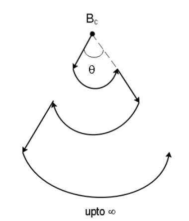
18 A current $i$ flows through an infinitely long wire having infinite bends as shown. The radius of the first curved section is \[a\] and the radii of successive curved portions each increase by a factor $\eta $. Find the magnetic field ${B_c}$.
Answer
232.8k+ views
Hint: In this solution, we will use the formula of the magnetic field generated by a current-carrying arc at its centre. Only the curved arcs will contribute to the magnetic fields since the straight bends are carrying a current in the direction of our point.
Formula used: In this solution, we will use the following formula:
Magnetic field due to curved arc: $B = \dfrac{{{\mu _0}I}}{{2a}}\dfrac{\theta }{{2\pi }}$ where$I$ is the current in the wire, $\theta $ is the angle subtended by the wire, $a$ is the radius of the wire.
Complete step by step answer:
In the diagram given to us, we can see that the wire is made up of curved portions and straight portions. Now, only the curved current-carrying portions will generate a magnetic field at the point of interest. This is because the straight wires are carrying current in a direction that passes through the point itself so there will be no magnetic field generated by the straight wire.
Now if the current in the first loop is $I$, the current in the next loop decreases by a factor $\eta $ so the current in the second loop will be $I/\eta $. Similarly, the current in the third loop will be $I/{\eta ^2}$, and so on.
Now the magnetic field due to one curved portion will be
$B = \dfrac{{{\mu _0}}}{{2a}}\dfrac{\theta }{{2\pi }}$
Since all the curves are at the same position (on top of each other), they will have the same radius, however, the current will be different. The current will also decrease in magnitude and the magnetic field generated by different loops will be different since the current flows in different directions.
Hence, the sum of all the individual magnetic fields will be
\[{B_{net}} = \dfrac{{{\mu _0}}}{{2r}}I\dfrac{\theta }{{2\pi }} - \dfrac{{{\mu _0}}}{{2a}}\dfrac{I}{\eta }\dfrac{\theta }{{2\pi }} + \dfrac{{{\mu _0}}}{{2a}}\dfrac{I}{{{\eta ^2}}}\dfrac{\theta }{{2\pi }} - \dfrac{{{\mu _0}}}{{2a}}\dfrac{I}{{{\eta ^3}}}\dfrac{\theta }{{2\pi }}....\]
Taking out $\dfrac{{{\mu _0}}}{{2a}}I\dfrac{\theta }{{2\pi }}$ common, we get
\[{B_{net}} = \dfrac{{{\mu _0}}}{{2a}}I\dfrac{\theta }{{2\pi }}\left( {1 - \dfrac{1}{\eta } + \dfrac{1}{{{\eta ^2}}} - \dfrac{1}{{{\eta ^3}}}...} \right)\]
The term in the bracket is an infinite geometric progression series so its sum will be $\dfrac{a}{{1 - m}}$ where $a = 1$ and $m = - \dfrac{1}{\eta }$. So,
\[{B_{net}} = \dfrac{{{\mu _0}}}{{2a}}I\dfrac{\theta }{{2\pi }}\left( {\dfrac{1}{{1 - \left( { - \dfrac{1}{\eta }} \right)}}} \right)\]
Or equivalently
\[{B_{net}} = \dfrac{{{\mu _0}}}{{4\pi a}}I\theta \left( {\dfrac{\eta }{{\eta + 1}}} \right)\]
Note: We must realize that the curved wires are not in-plane and are actually below each other. If the wires were in one plane, the radius of the curved regions would also eventually increase.
Recently Updated Pages
JEE Main 2023 April 6 Shift 1 Question Paper with Answer Key
JEE Main 2023 April 6 Shift 2 Question Paper with Answer Key
JEE Main 2023 (January 31 Evening Shift) Question Paper with Solutions [PDF]
JEE Main 2023 January 30 Shift 2 Question Paper with Answer Key
JEE Main 2023 January 25 Shift 1 Question Paper with Answer Key
JEE Main 2023 January 24 Shift 2 Question Paper with Answer Key
Trending doubts
JEE Main 2026: Session 2 Registration Open, City Intimation Slip, Exam Dates, Syllabus & Eligibility
JEE Main 2026 Application Login: Direct Link, Registration, Form Fill, and Steps
Understanding the Angle of Deviation in a Prism
Hybridisation in Chemistry – Concept, Types & Applications
How to Convert a Galvanometer into an Ammeter or Voltmeter
Understanding Uniform Acceleration in Physics
Other Pages
JEE Advanced Marks vs Ranks 2025: Understanding Category-wise Qualifying Marks and Previous Year Cut-offs
Dual Nature of Radiation and Matter Class 12 Physics Chapter 11 CBSE Notes - 2025-26
Understanding the Electric Field of a Uniformly Charged Ring
JEE Advanced Weightage 2025 Chapter-Wise for Physics, Maths and Chemistry
Derivation of Equation of Trajectory Explained for Students
Understanding Electromagnetic Waves and Their Importance