


Introduction to Matrices
Matrices are one of the most exciting, simple, and important concepts in Mathematics. This chapter is totally new from the student's perspective, as it appears right after the 11th. As a result, some students may find Matrices difficult to comprehend and solve problems with at first. However, as you solve more questions in this chapter and become more comfortable with the concepts and the chapter as a whole, you will discover that this is one of the easier chapters.
Matrix, types of matrices, operations on matrices, transpose of a matrix, application of matrices, some of the solved examples, and some previous year questions will be discussed in this article.
Important Topics of Matrices
Matrices
Operation on Matrices
Types of Matrices
Transpose of Matrix
Matrix Multiplication
Inverse Matrix
Inverse of 3 by 3 Matrix
Important Chapters of Matrices
What is the Matrix?
In Mathematics, a matrix (plural matrices) is a rectangular array of numbers, symbols, or expressions arranged in rows and columns. When writing matrices, box brackets are usually applied. The horizontal and vertical lines of entries in a matrix are referred to as rows and columns, respectively. The number of rows and columns in a matrix determines the size of the matrix. A matrix with m rows and n columns is called an m × n matrix or m-by-n matrix, while m and n are called its dimensions. The dimensions of the following matrix are 2 x 3 up(read “two by three”), because there are two rows and three columns.
$A={\displaystyle {\begin{bmatrix}1&9&-13\\20&5&-6\end{bmatrix}}}$
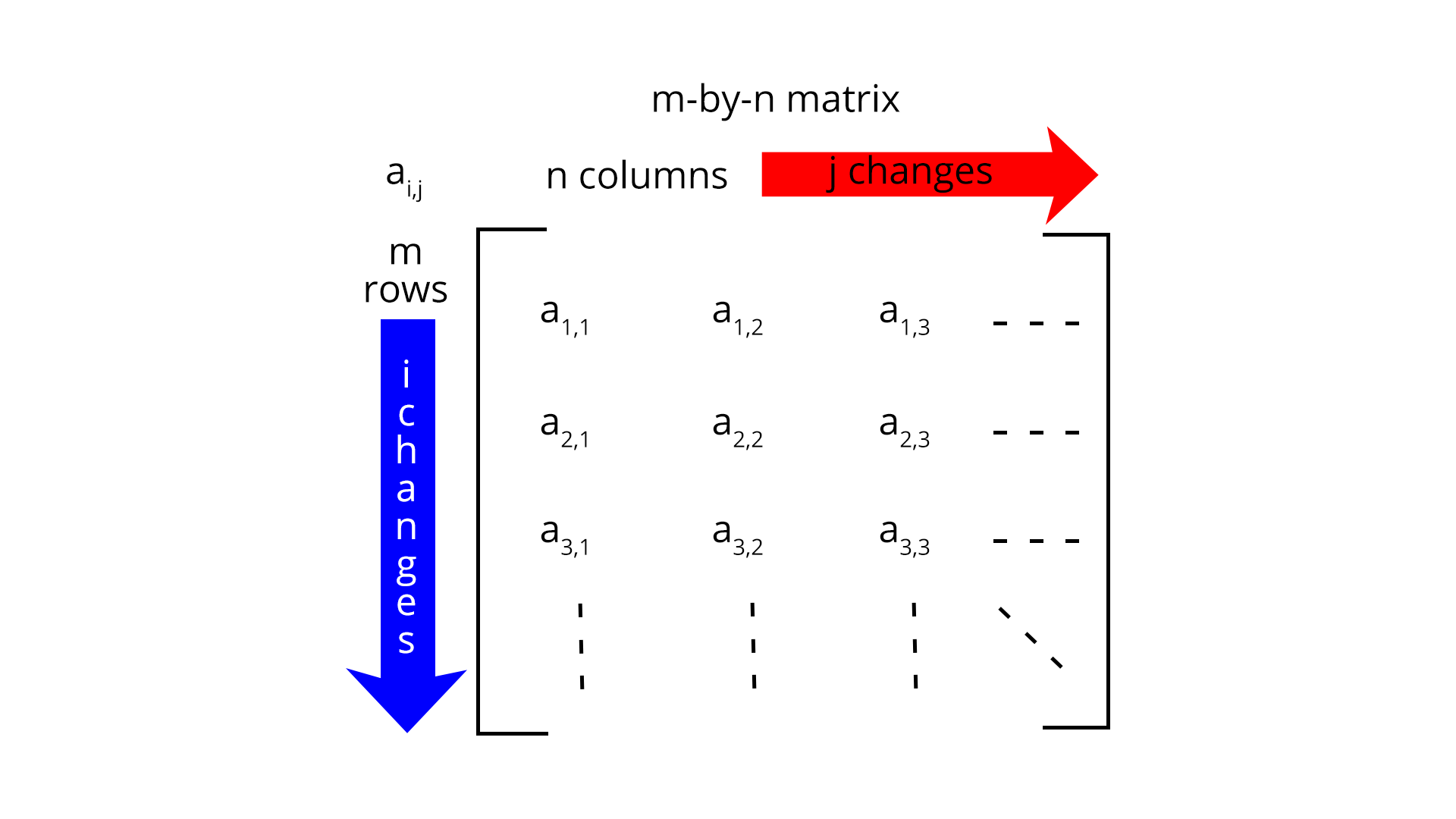
Image: Matrix dimension - Each element of a matrix is often denoted by a variable with two subscripts.
The elements or entries of a matrix are the individual items (numbers, symbols, or phrases) that make up the matrix.
Two matrices can be added or removed element by element as long as they are the same size (have the same number of rows and columns). The rule for matrix multiplication, on the other hand, is that two matrices can only be multiplied if the first's number of columns equals the second's number of rows. A scalar from the related field can be multiplied element-by-element by any matrix.
Row vectors are matrices with a single row, and column matrices are matrices with a single column. A square matrix is a matrix with the same number of rows and columns. A matrix with no rows or columns, known as an empty matrix, is beneficial in particular situations, such as computer algebra applications.
Types of Matrix
Row Matrix - A matrix having one row is called a row matrix.
Column Matrix - A matrix having one column is called a column matrix.
Square Matrix - A matrix of order m×n is called a square matrix if m = n.
Zero Matrix - A = [aij] m×n is called a zero matrix if aij = 0 for all i and j.
Upper triangular Matrix - A = [aij]m×n is said to be upper triangular if aij= 0 for i > j.
Lower triangular Matrix - A = [aij]m×n is said to be lower triangular if aij = 0 for i < j.
Diagonal Matrix - A square matrix [aij]m×n is said to be diagonal, if aij = 0 for i ≠ j.
Scalar Matrix - A diagonal matrix A = [aij]m×n is said to be scalar, if aij = k for i = j.
Unit Matrix (Identity matrix) - A diagonal matrix A = [aij]n is a unit matrix if aij = 1 for i = j.
Comparable Matrices - Two matrices A and B are said to be comparable if they have the same order.
Matrix Algebra
Matrix Addition and Subtraction
Matrixes are used to represent systems or to list data. We can execute operations on matrices since the elements are integers. By adding/deleting corresponding entries, we can add or subtract the given matrices.
The entries must match in order to accomplish this. As a result, adding and subtracting matrices is only conceivable when their dimensions are the same. Because matrix addition is both commutative and associative, the following holds true:
$\displaystyle A+B=B+A $
$\displaystyle (A+B)+C=A+(B+C)$
Adding matrices is a simple process. Simply multiply each element in the first matrix by the number in the second matrix.
$\displaystyle \begin {pmatrix} 1 & 2 & 3 \\ 4 & 5 & 6 \end{pmatrix}+\begin{pmatrix} 10 & 20 & 30 \\ 40 & 50 & 60 \end{pmatrix}=\begin {pmatrix} 11 & 22 & 33 \\ 44 & 55 & 66 \end {pmatrix}$
Note that the element in the first matrix, 1, adds to the element X11 in the second matrix, 10, to produce element X11 in the resultant matrix, 11. Also note that both matrices being added are 2 x 3, and the resulting matrix is also 2 x 3.
And, the 2 matrices of the different dimensions cannot be added.
As you know, the subtracting works much the same way except that you subtract instead of adding.
$\displaystyle \begin{pmatrix} 10 & -20 & 30 \\ 40 & 50 & 60 \end{pmatrix}-\begin{pmatrix} 1 & -2 & 3 \\ 4 & -5 & 6 \end{pmatrix}=\begin{pmatrix} 9 & -18 & 27 \\ 36 & 55 & 54 \end{pmatrix}$
It's worth repeating that the new matrix has the same dimensions as the originals and that you can't subtract two matrices of different dimensions. When subtracting signed numbers, be cautious.
Matrix Multiplication
1. Scalar Multiplication
Scalar multiplication of a real Euclidean vector by a positive real number multiplies the magnitude of the vector without changing its direction in an intuitive geometrical context. What does it mean to multiply a number by 3? It means you add the number to itself 3 times. Multiplying a matrix by 3 means the same thing; you add the matrix to itself 3 times or simply multiply each element by that constant.
$\displaystyle 3\cdot \begin{pmatrix} 1 & 2 & 3 \\ 4 & 5 & 6 \end{pmatrix}=\begin{pmatrix} 3 & 6 & 9 \\ 12 & 15 & 18 \end{pmatrix}$
The resulting matrix has the same dimensions as the original and the Scalar multiplication has the following properties:
Left and right distributivity: $(c+d)\textbf{M} = \textbf{M}(c+d) = \textbf{M}c+\textbf{M}d$
Associativity: $(cd)\textbf{M} = c(d\textbf{M})$
Identity: $1\textbf{M} = \textbf{M}$
Null: $0\textbf{M} = \textbf{0}$
Additive inverse: $(-1)\textbf{M} = -\textbf{M}$
2. Multiplication with Another Matrix
When multiplying matrices, the elements of the first matrix's rows are multiplied by the elements of the second matrix's columns.
If A is an n x m matrix and B is an m x p matrix, the result AB of their multiplication is an n x p matrix defined only if the number of columns m in A is equal to the number of rows m in B. Before multiplying the matrices, double-check that this is the case, as there would be "no solution" otherwise.
General Definition and Process: Matrix Multiplication
Matrix multiplication is simply multiplying every element of each row of the first matrix times every element of each column in the second matrix, whereas scalar multiplication is simply multiplying a value through all the elements of a matrix. Although scalar multiplication is significantly easier than matrix multiplication, there is a pattern.
When multiplying matrices, the elements of the first matrix's rows are multiplied by the elements of the second matrix's columns. The resultant matrix's entries are computed one by one.
For 2 matrices, the final position of the product obtained is shown below:
$\displaystyle \begin{bmatrix} { a }_{ 11 } & { a }_{ 12 } \\ \cdot & \cdot \\ { a }_{ 31 } & { a }_{ 32 } \\ \cdot & \cdot \end{bmatrix}\begin{bmatrix} \cdot & { b }_{ 12 } & { b }_{ 13 } \\ \cdot & { b }_{ 22 } & { b }_{ 23 } \end{bmatrix}=\begin{bmatrix} \cdot & x_{ 12 } & \cdot \\ \cdot & \cdot & \cdot \\ \cdot & \cdot & { x }_{ 33 } \\ \cdot & \cdot & \cdot \end{bmatrix}$
The values at the intersections marked with circle are:
$\displaystyle {x}_{12}=({a}_{11},{a}_{12}) \cdot ({b}_{12},{b}_{22})=({a}_{11} {b}_{12}) +({a}_{12} {b}_{22})$
$\displaystyle {x}_{33}=({a}_{31},{a}_{32}) \cdot ({b}_{13},{b}_{23})=({a}_{31} {b}_{13}) +({a}_{32} {b}_{23})$
Matrices Rules of Algebra
Matrix algebra follows a set of rules for addition and multiplication. Consider the following three square matrices: A, B, and C. A' is the inverse of A, and A-1 is the transpose of A. R is a real number, and I is the identity matrix.
Now according to the laws of matrices,
A+B = B+A $\rightarrow$ Commutative Law of Addition
A+B+C = A +(B+C) = (A+B)+C $\rightarrow$Associative law of addition
ABC = A(BC) = (AB)C $\rightarrow$ Associative law of multiplication
A(B+C) = AB + AC $\rightarrow$ Distributive law of matrix algebra
R(A+B) = RA + RB
The inverse rules of matrices are given below:
AI = IA = A
AA-1 = A-1A = I
(A-1)-1 = A
(AB)-1 = B-1A-1
(ABC)-1 = C-1B-1A-1
(A’)-1 = (A-1)’
Transpose of a Matrix
Let A = [aij]m×n. Then, A’ or AT, the transpose of A, is defined as A’ = [aji]n×m .
(i) (A’)’ = A
(ii) (λA)’ = λA’
(iii) (A+B)’ = A’+B’
(iv) (A-B)’ = A’-B’
(v) (AB)’ = A’B’
(vi) For a square matrix A, if A’ = A, then Matrix A is said to be a symmetric matrix.
(vii) For a square matrix A, if A’ = -A, then Matrix A is said to be a skew symmetric matrix.
Application of Matrices
Matrices are used in our day-to-day life in many areas. Some of the uses of matrices in daily life are given below:
Encryption – Encryption is a popular application of matrix in everyday life. We use it to jumble data for security reasons, and we need matrices to encode and decode it. There is a key that aids in the encoding and decoding of data generated by matrices.
Games, Especially 3D Games – Matrices are used in games, for example, in 3D space, we use it to change the object. They convert it from a three-dimensional matrix to a two-dimensional matrix as needed.
Economics and Business – To research a company's trends, stocks, and other assets, as well as to develop business models.
Construction – The building industry is another common application of matrices in real life. Have you ever seen a building that is straight on the outside but the architects strive to change the structure on the outside? Matrices can be used to do this. A matrix is made up of rows and columns, and the number of rows and columns in a matrix can be changed. Matrices can assist in the support of a variety of historical structures.
Animation – It can aid in the creation of more exact and accurate animations.
List of Formulas
Solved Examples
Example 1: Given $\begin{array}{l}A= \begin{bmatrix} 3 &-5 \\ -1 &7 \end{bmatrix}\end{array} $ and $\begin{array}{l}B= \begin{bmatrix} 1 &4 \\ 8 &3 \end{bmatrix}\end{array} $ find A + B.
Solution:
Given, $\begin{array}{l}A= \begin{bmatrix} 3 &-5 \\ -1 &7 \end{bmatrix}\end{array} $
and $\begin{array}{l}B= \begin{bmatrix} 1 &4 \\ 8 &3 \end{bmatrix}\end{array} $
Addition of A and B is: $\begin{array}{l}A+B= \begin{bmatrix} 3 &-5 \\ -1 &7 \end{bmatrix}+ \begin{bmatrix} 1 &4 \\ 8 &3 \end{bmatrix}\\ =\begin{bmatrix} 3+1 &-5+4 \\ -1+8 &7+3 \end{bmatrix}\\=\begin{bmatrix} 4 &-1 \\ 7 &10 \end{bmatrix}\end{array} $
Example 2: If $\begin{array}{l}P= \begin{bmatrix} 5 &4 \\ 2 &9 \end{bmatrix}\end{array} $ and $\begin{array}{l}Q= \begin{bmatrix} 1 &5 \\ 0&2 \end{bmatrix}\end{array} $, then find P-Q.
Solution:
Given, $\begin{array}{l}P= \begin{bmatrix} 5 &4 \\ 2 &9 \end{bmatrix}\end{array} $ and
$\begin{array}{l}Q= \begin{bmatrix} 1 &5 \\ 0&2 \end{bmatrix}\end{array} $
Subtraction of the matrices P and Q is: $\begin{array}{l}A-B= \begin{bmatrix} 5 &4 \\ 2 &9 \end{bmatrix}- \begin{bmatrix} 1 &5 \\ 0 &2 \end{bmatrix}\\ =\begin{bmatrix} 5-1 &4-5 \\ 2-0 &9-2 \end{bmatrix}\\=\begin{bmatrix} 4 &-1 \\ 2 &7 \end{bmatrix}\end{array} $
Solved Problem of Previous Year Question Paper
Question 1: $\begin{array}{l}\left[ \begin{matrix} 1 & 0 & 0 \\ 0 & 1 & 1 \\ 0 & -2 & 4 \\ \end{matrix} \right];\,\,I=\left[ \begin{matrix} 1 & 0 & 0 \\ 0 & 1 & 0 \\ 0 & 0 & 1 \\ \end{matrix} \right]\end{array} $
$\begin{array}{l}A^{-1}=\frac{1}{6}(A^{2}+cA+dI)\end{array} $ where c, d ∈ R, then pair of values (c, d) are __________.
Solution:
Given
$\begin{array}{l}A=\left[ \begin{matrix} 1 & 0 & 0 \\ 0 & 1 & 1 \\ 0 & -2 & 4 \\ \end{matrix} \right]\end{array} $
$\begin{array}{l}A^{-1}=\frac{1}{6}\left[ \begin{matrix} 6 & 0 & 0 \\ 0 & 4 & -1 \\ 0 & 2 & 1 \\ \end{matrix} \right]\end{array} $
$\begin{array}{l}A^2=\left[ \begin{matrix} 1 & 0 & 0 \\ 0 & 1 & 1 \\ 0 & -2 & 4 \\ \end{matrix} \right]\,\left[ \begin{matrix} 1 & 0 & 0 \\ 0 & 1 & 1 \\ 0 & -2 & 4 \\ \end{matrix} \right]=\left[ \begin{matrix} 1 & 0 & 0 \\ 0 & -1 & 5 \\ 0 & -10 & 14 \\ \end{matrix} \right]\end{array} $
$\begin{array}{l} cA=\left[ \begin{matrix} c & 0 & 0 \\ 0 & c & c \\ 0 & -2c & 4c \\ \end{matrix} \right]\end{array} $
$\begin{array}{l} dI=\left[ \begin{matrix} d & 0 & 0 \\ 0 & d & 0 \\ 0 & 0 & d \\ \end{matrix} \right]\end{array} $
Therefore, by
$\begin{array}{l}A^{-1}=\frac{1}{6}(A^2+cA+dI)\end{array} $
⇒ 6 = 1 + c + d, (by equality of matrices)
So, (-6, 11) satisfy the relation.
Question 2: If $\begin{array}{l} P=\left[ \begin{matrix} \frac{\sqrt{3}}{2} & \frac{1}{2} \\ -\frac{1}{2} & \frac{\sqrt{3}}{2} \\ \end{matrix} \right],\,A=\left[ \begin{matrix} 1 & 1 \\ 0 & 1 \\ \end{matrix} \right]\end{array} $ and Q = PAPT, then P (Q2005)PT equal to ________.
Solution:
If Q = PAPT, PTQ = APT,
(as PPT = I) PT Q2005 P = A PT Q2004 P
= A2 PT Q2003 P
= A3 PT Q2002 P
= A2004 PT (QP)
= A2004 PT (PA) (Q = PAPT ⇒ QP = PA)
= A2005
A2005 = $\begin{array}{l}\left[ \begin{matrix} 1 & 2005 \\ 0 & 1 \\ \end{matrix} \right]\end{array} $
Question 3: If $\begin{array}{l}A=\left[ \begin{matrix} \alpha & 0 \\ 1 & 1 \\ \end{matrix} \right] and \ B=\left[ \begin{matrix} 1 & 0 \\ 5 & 1 \\ \end{matrix} \right]\end{array} $
then value of α for which A2 = B is
A. 1
B. -1
C. 4
D. No real values
Solution:
$\begin{array}{l}A^2=\left[ \,\begin{matrix} \alpha & 0 \\ 1 & 1 \\ \end{matrix}\, \right]\,\left[ \,\begin{matrix} \alpha & 0 \\ 1 & 1 \\ \end{matrix}\, \right]=\left[ \,\begin{matrix} {{\alpha }^{2}} & 0 \\ \alpha +1 & 1 \\ \end{matrix}\, \right]\end{array} $
Clearly, no real value of a.
Practice Questions
Q1. Let $\mathrm{M}$ and $\mathrm{N}$ be two $3 \times 3$ non-singular skew-symmetric matrices such that $\mathrm{MN}=\mathrm{NM}$. If $\mathrm{P}^{\mathrm{T}}$ denotes the transpose of $\mathrm{P},$ then $\mathrm{M}^{2} \mathrm{N}^{2}\left(\mathrm{M}^{\mathrm{T}} \mathrm{N}\right)^{-1}\left(\mathrm{MN}^{-1}\right)^{\mathrm{T}}$ is equal to –
(A). $\mathbf{M}^{2}$
(B). $-N^{2}$
(C). $-M^{2}$
(D). MN
Q2. Let $\omega \neq 1$ be a cube root of unity and $S$ be the set of all non-singular matrices of the form $\left[\begin{array}{lll}{1} & {a} & {b} \\ {\omega} & {1} & {c} \\ {\omega^{2}} & {\omega} & {1}\end{array}\right],$ where each of a,b and $c$ is either $\omega$ or $\omega^{2} .$ Then the number of distinct matrices in the set $\mathrm{S}$ is-
(A). 2
(B). 6
(C). 4
(D). 8
Answers: 1-C, 2-A
Conclusion
Matrices can be used to write and work with many linear equations, or a system of linear equations, in a compact manner. When it comes to linear transformations, often known as linear maps, matrices and matrix multiplication show their real features. We went through matrix definitions, types, and algebraic operations in this article. In addition, for a better understanding of the chapter, we went over some of the solved examples and previous year's questions.
FAQs on JEE Chapter - Matrices
1. What is the contribution of the chapter Matrix in JEE?
Every year, at least 1-3 problems from this chapter will appear in JEE Main and other tests, and the concept of this chapter will appear in many other chapters, such as integral and differential calculus. The axis-transformation notion will be based on the concepts discussed in this chapter.
2. How important are the chapter Matrices for JEE Advanced?
The most basic chapters in entrance exams are matrices and determinants; however, they are critical in JEE Main and Advanced. Matrices are also easier to use for solving systems of equations than determinants. If you grasp the determinant first, solving matrices becomes a lot easier. Determinants are also more widely employed in Mathematics than matrices.
3. What are matrices used for?
Matrices are commonly used in geometry to express and represent geometric transformations (such as rotations) and coordinate changes. Many computer difficulties in numerical analysis are solved by reducing them to a matrix calculation, which frequently requires computing with matrices of enormous dimensions.