


Find Complete Probability Class 10 Questions and Answers for Better Understanding
NCERT Solutions For Class 10 Maths - Probability help you learn about chances and outcomes. This chapter teaches you how to find the possibility of events happening. Probability is used in games, sports, and real life situations.
 Table of Content
Key points covered:
• Solutions for finding probability of single and multiple events
• Step-by-step answers for theoretical and experimental probability
• Practice questions with detailed explanations for all exercises
• Easy methods to solve probability word problems
Vedantu's NCERT Solutions make every problem simple to solve. Download the NCERT Solutions PDF for free and start practicing today! These solutions save time during exam preparation. Visit NCERT Solutions Class 10 Maths for more chapter-wise help and practice materials.
Access Exercise Wise NCERT Solutions for Chapter 14 Maths Class 10
NCERT Solutions For Class 10 Maths Chapter 14 Probability - 2026-27
Exercise 14.1: This exercise involves solving word problems by paying close attention to key terms like event, sample space, and favourable outcome definitions. Break down complex problems into simpler events and apply the relevant rules.
Access NCERT Solutions for Class 10 Maths Chapter 14 – Probability
Exercise 14.1
1. Complete the following statements:
i. Probability of an event E + Probability of the event ‘not E’ = _____.
Ans:
If the probability of an event be $p$, then the probability of the ‘not event’ will be, $1-p$ . Thus, the sum will be, $p+1-p=1$.
ii. The probability of an event that cannot happen is _____. Such an event is called _____.
Ans:
The probability of an event that cannot happen is always $0$.
iii. The probability of an event that is certain to happen is _____. Such an event is called _____.
Ans:
The probability of an event that is certain to happen is $1$ . Such an event is called, sure event.
iv. The sum of the probabilities of all the elementary events of an experiment is _____.
Ans:
The sum of the probabilities of all the elementary events of an experiment is $1$.
v. The probability of an event is greater than or equal to and less than or
equal to _____.
Ans:
The probability of an event is greater than or equal to $0$ and less than or equal to $1$ .
2. Which of the following experiments have equally likely outcomes? Explain.
i. A driver attempts to start a car. The car starts or does not start.
Ans:
Equally likely outcomes defined as the outcome when each outcome is likely to occur as the others. So, the outcomes are not equally likely outcome.
ii. A player attempts to shoot a basketball. She/he shoots or misses the shot.
Ans:
The outcomes are not equally likely outcome.
(iii) A trial is made to answer a true-false question. The answer is right or wrong.
Ans:
The outcomes are equally likely outcome.
(iv) A baby is born. It is a boy or a girl.
Ans:
The outcomes are not equally likely outcome.
3. Why is tossing a coin considered to be a fair way of deciding which team should get the ball at the beginning of a football game?
Ans:
We already know the fact that a coin has only two sides, head and tail. So, when we toss a coin, it will either give us the result head or tail. There is no chance of the coin landing on his edge. And on the other hand, the chances of getting head and tail are also just the same. So, it can be concluded that the tossing of a coin is a fair way to decide the utcome, as it can not be biased and both teams will have the same chance of winning.
4. Which of the following cannot be the probability of an event?
(A) $\frac{2}{3}$
Ans:
The probability of an event have to always be in the range of $[0,1]$ .
Now, let us the check the given values.
We can see, $\frac{2}{3}=0.67$ . This is in the given range. It can be a probability of an event.
(B) $-1.5$
Ans:
We can see, $-1.5$ , which is a negative number and not inside the given range. It can not be a probability of an event.
(C) $15%$
Ans:
We can see, $15%=\frac{15}{100}=0.15$ . This is in the given range of $[0,1]$ . It can be a probability of an event.
(D) $0.7$
Ans:
We can see, $0.7$ , which is in the given range. It can be a probability of an event.
5. If $P(E)=0.05$ , what is the probability of an event ‘not $E$’?
Ans:
The sum of the probabilities of all events in always $1$ .
Thus, if $P(E)=0.05$ , the probability of the event ‘not E’ is, $1-0.05=0.95$.
6. A bag contains lemon flavored candies only. Malini takes out one candy without looking into the bag. What is the probability that she takes out
i.an orange flavored candy?
Ans:
There is no orange candy available in the bag, so, the probability of taking out an orange flavored candy is $0$.
(ii) a lemon flavored candy?
Ans:
All the candies in the bag are lemon flavored candies only. Thus, any candy Malini takes out will be a lemon flavored candy.
So, the probability of taking out a lemon flavored candy is $1$.
7. It is given that in a group of 3 students, the probability of $2$ students not having the same birthday is $0.992$ . What is the probability that the $2$ students have the same birthday?
Ans:
It is provided to us that, probability of 2 students not having the same birthday is, $0.992$ .
So,$P(2\text{ students }\text{having }\text{the}\text{ same}\text{ birthday})+P(\text{2}\text{ students }\text{not }\text{having }\text{the}\text{ same}\text{ birthday})=1$
$\Rightarrow P(\text{2}\text{ students}\text{ having}\text{ the }\text{same}\text{ birthday})+0.992=1$
Simplifying further,
$P(2 \text{students having the same birthday})=0.008$.
8. A bag contains $3$ red balls and $5$ black balls. A ball is drawn at random from the bag. What is the probability that the ball drawn is (i) red ?
Ans:
The bag is having $3$ red balls and $5$ black balls.
Now, the probability of getting a red ball will be, $\frac{number\,of\,red\,balls}{total\,number\,of\,balls}$ .
Putting the values, we get, $\frac{3}{3+5}=\frac{3}{8}$ .
(ii) not red?
Ans:
And, the probability of getting a red ball will be, $1-\frac{number\,of\,red\,balls}{total\,number\,of\,balls}$.
Again, putting the values, $1-\frac{3}{8}=\frac{5}{8}$.
9. A box contains $5$ red marbles, $8$ white marbles and green marbles. One marble is taken out of the box at random. What is the probability that the marble taken out will be (i) red ?
Ans:
The box is containing, $5$ red marbles, $8$ white marbles and green marbles.
The probability of getting a red marble will be, $\frac{number\,of\,red\,marbles}{total\,number\,of\,marbles}$
Putting the values, $\frac{5}{5+8+4}=\frac{5}{17}$.
(ii) white ?
Ans:
Again, the probability of getting a white marble will be, $\frac{number\,of\,white\,marbles}{total\,number\,of\,marbles}$
Putting the values, $\frac{8}{5+8+4}=\frac{8}{17}$.
(iii) not green?
Ans:
And, the probability of getting a green marble will be, $\frac{number\,of\,green\,marbles}{total\,number\,of\,marbles}$.
Putting the values, $\frac{4}{5+8+4}=\frac{4}{17}$ .
So, the probability of the marble not being green will be, $1-\frac{4}{17}=\frac{13}{17}$.
10. A piggy bank contains hundred $50$ p coins, fifty ` $1$ coins, twenty ` $2$ coins and ten ` $5$ coins. If it is equally likely that one of the coins will fall out when the bank is turned upside down, what is the probability that the coin (i) will be a $50$ p coin ?
Ans:
We are provided with the fact that, the piggy bank contains, hundred $50$ p coins, fifty $1$ rs coins, twenty $2$ rs coins and ten $5$ rs coins.
So, the total number of coins, $100+50+20+10=180$ .
Thus, the probability of drawing a $50$ p coin, $\frac{100}{180}=\frac{5}{9}$.
ii. will not be a ` $5$ coin?
Ans:
Similarly, the probability of drawing a $5$ rs coin, $\frac{10}{180}=\frac{1}{18}$ .
Thus, the probability of not getting a $5$ rs coin, $1-\frac{1}{18}=\frac{17}{18}$ .
11.
Gopi buys a fish from a shop for his aquarium. The shopkeeper takes out one fish at random from a tank containing $5$ male fish and $8$ female fish (see Fig. 15.4). What is the probability that the fish taken out is a male fish?

Ans:
The total number of fishes in the tank, $5+8=13$ .
Thus, the probability of getting a male fish, $\frac{no\,of\,male\,fishes}{total\,no\,of\,fishes}=\frac{5}{13}$.
12. A game of chance consists of spinning an arrow which comes to rest pointing at one of the numbers $1,2,3,4,5,6,7,8$ (see Fig. 15.5), and these are equally likely outcomes. What is the probability that it will point at
(i)$8?$
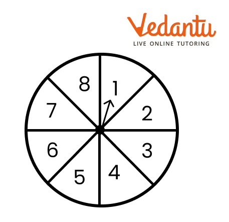
Ans:
We can see, there are $8$ numbers on spinner then the total number of favorable outcome is $8$ .
Thus, the probability of getting the number $8$ is, $\frac{no\,of\,digit\,8\,on\,the\,spinner}{total\,number\,of\,digits}=\frac{1}{8}$.
(ii) $\text{an odd number?}$
Ans:
There are 4 odd digits, $1,3,5,7$ .
Thus, the probability of getting an odd number is,
$\frac{no\,of\,odd\,digits\,}{total\,number\,of\,digits}=\frac{4}{8}=\frac{1}{2}$ .
(iii) $\text{a number greater than 2?}$
Ans:
There are 6 numbers greater than 2, say $3,4,5,6,7,8$ .
Thus, the probability of getting a number greater than 2, $\frac{no\,of\,digits\,greater\,than\,2\,on\,the\,spinner}{total\,number\,of\,digits}=\frac{6}{8}=\frac{3}{4}$.
(iv) $\text{a number less than 9}$$?$
Ans:
As we can see, every number in the spinner is less than $9$ , thus, we get,
The probability of getting a number less than $9$ , will be, $1$.
13. A die is thrown once. Find the probability of getting (i) a prime number;
Ans:
There is $6$ results can be obtained from a dice.
There are 3 prime numbers, $2,3,5$ among those results.
Thus, the probability of getting a prime number,$=\frac{\text{no }\text{of }\text{prime }\text{numbers }\text{in }\text{a}\text{ dice}}{\text{total}\text{ numbers}\text{ on }\text{dice}}=\frac{3}{6}=\frac{1}{2}$
(ii) a number lying between $2$ and $6$
Ans:
There are 3 numbers between 2 and 6, 3,4,5.
Thus, the probability of getting a number between 2 and 6,
$=\frac{\text{no }\text{of }\text{numbers }\text{between }\text{2}\text{ and}\text{ 6 }\text{in}\text{ a}\text{ dice}}{\text{total}\text{ numbers }\text{on}\text{ dice}}=\frac{3}{6}=\frac{1}{2}$
(iii) an odd number.
Ans:
There are 3 odd numbers among the results, 1,3,5.
Thus, the probability of getting a odd number,
$=\frac{\text{no }\text{of}\text{ odd }\text{numbers}\text{ between}\text{ in }\text{a }\text{dice}}{\text{total}\text{ numbers }\text{on}\text{ dice}}=\frac{3}{6}=\frac{1}{2}$
14. One card is drawn from a well-shuffled deck of 52 cards. Find the probability of getting
(i) a king of red color
Ans:
We know there are 52 numbers in the deck.
There are 2 kings of red color in the deck.
Thus, the probability,
$=\frac{total\,number\,of\,red\,kings}{total\,number\,of\,cards}=\frac{2}{52}=\frac{1}{26}$
(ii) a face cards
Ans:
There are 12 face cards in the deck.
Thus, the probability,
$=\frac{total\,number\,of\,face\,cards}{total\,number\,of\,cards}=\frac{12}{52}=\frac{3}{13}$
(iii) a red face cards
Ans:
There are 6 red face cards in the deck.
Thus, the probability,
$=\frac{total\,number\,of\,red\,face\,cards}{total\,number\,of\,cards}=\frac{6}{52}=\frac{3}{26}$
(iv) the jack of hearts
Ans:
There are 1 jack of hearts card in the deck.
Thus, the probability,
$=\frac{total\,number\,of\,red\,face\,cards}{total\,number\,of\,cards}=\frac{1}{52}$
(v) a spade
Ans:
There are 13 spade cards in the deck.
Thus, the probability,
$=\frac{total\,number\,of\,spade\,cards}{total\,number\,of\,cards}=\frac{13}{52}=\frac{1}{4}$
(vi) the queen of diamonds
Ans:
There are 1 queen of diamonds card in the deck.
Thus, the probability,
$=\frac{total\,number\,of\,red\,face\,cards}{total\,number\,of\,cards}=\frac{1}{52}$
15. Five cards—the ten, jack, queen, king and ace of diamonds, are well-shuffled with their face downwards. One card is then picked up at random.
(i) What is the probability that the card is the queen?
Ans:
There are total 5 cards given in our deck.
Thus, the probability of getting a queen card among the 5 cards,
\[=\frac{number\,of\,queen}{number\,of\,total\,cards}=\frac{1}{5}\]
(ii) If the queen is drawn and put aside, what is the probability that the second card picked up is (a) an ace? (b) a queen?
Ans:
Now, the queen is put aside, so there will be 4 cards left.
a. Thus, the probability of getting a queen card among the 5 cards,
\[=\frac{number\,of\,ace}{number\,of\,total\,cards}=\frac{1}{4}\]
b. There are no queen cards left in the deck.
Thus, the probability of getting a queen card among the 4 cards,
\[=\frac{number\,of\,queen}{number\,of\,total\,cards}=\frac{0}{4}=0\]
16. 12 defective pens are accidentally mixed with 132 good ones. It is not possible to just look at a pen and tell whether or not it is defective. One pen is taken out at random from this lot. Determine the probability that the pen taken out is a good one.
Ans:
There are total (132+12)=144 number of pens in the lot.
And also there are 132 good pens in the given collection.
Thus, the probability of getting a good pen,
$=\frac{number\,of\,good\,pens}{number\,of\,total\,pens}=\frac{132}{144}=\frac{11}{12}$
17. A lot of 20 bulbs contain 4 defective ones. One bulb is drawn at random from the lot. What is the probability that this bulb is defective?
Ans:
There are 4 defective bulbs among 20 bulbs.
Thus, the probability of getting a defective bulb,
$=\frac{number\,of\,defective\,bulb}{number\,of\,total\,bulb}=\frac{4}{20}=\frac{1}{5}$
ii. Suppose the bulb drawn in (i) is not defective and is not replaced. Now one bulb is drawn at random from the rest. What is the probability that this bulb is not defective ?
Ans:
After the first draw, there are 19 bulbs left in the lot. Again, as the bulb was a non-defective bulb, the total non-defective bulbs are 15.
Therefore, the probability of not getting a defective bulb this time,
$=\frac{15}{19}$ .
18. A box contains 90 discs which are numbered from $1$ to $90$ . If one disc is drawn at random from the box, find the probability that it bears (i) a two-digit number.
Ans:
There are 81 two digit numbers between 1 to 90.
Thus, the probability of getting a two digit number in the draw,
$=\frac{the\,total\,number\,of\,two\,digit\,numbers}{total\,numbers}=\frac{81}{90}=\frac{9}{10}$
(ii) a perfect square number
Ans:
The number of perfect square numbers between 1 to 90.
Thus, the probability of getting a perfect number in the draw,
$=\frac{the\,total\,number\,of\,perfect\,number}{total\,numbers}=\frac{9}{90}=\frac{1}{10}$
(iii) a number divisible by $5$.
Ans:
The number of numbers divisible by 5, 18.
Thus, the probability of getting a number divisible by 5 in the draw,
$=\frac{the\,total\,number\,of\,number\,divisible\,by\,5}{total\,numbers}=\frac{18}{90}=\frac{1}{5}$
19. A child has a die whose six faces show the letters as given below: A, A, B, C, D, E. The die is thrown once. What is the probability of getting

(i) A?
Ans:
There are two A’s in the six faces, so, the probability of getting an A,
$=\frac{total\,number\,of\,A's}{total\,number\,of\,sides}=\frac{2}{6}=\frac{1}{3}$
(ii) D?
Ans:
There are one D in the six faces, so, the probability of getting an D,
$=\dfrac{total\,number\,of\,D's}{total\,number\,of\,sides}=\dfrac{1}{6}$
20. Suppose you drop a die at random on the rectangular region shown in Fig. 15.6. What is the probability that it will land inside the circle with diameter 1m?
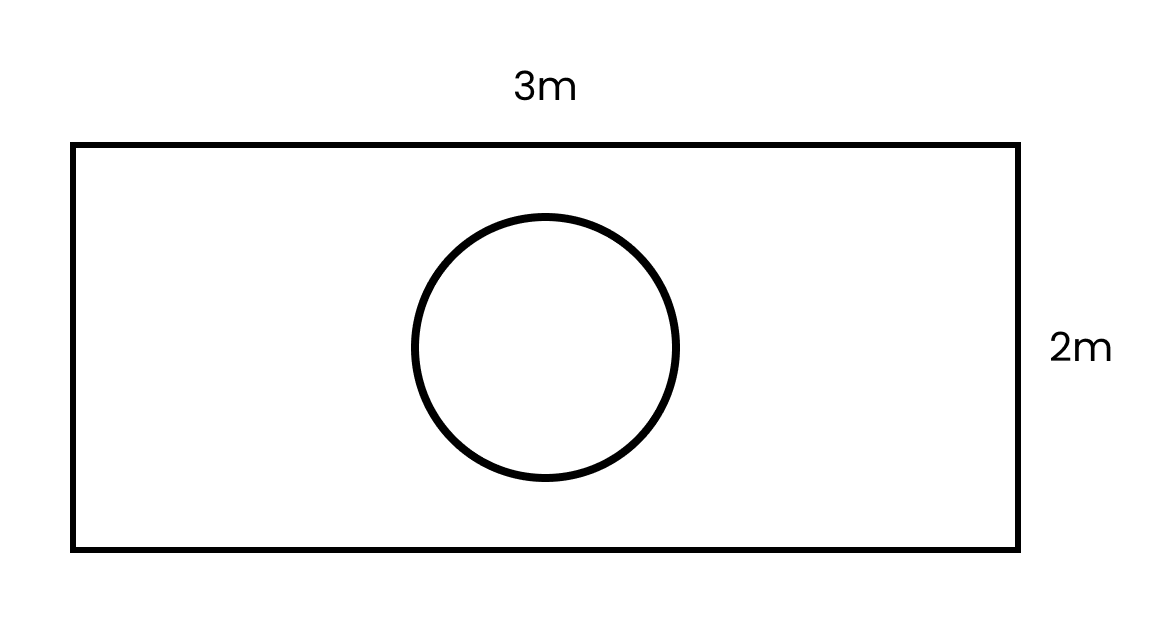
Ans:
It is given that it is a rectangle with sides 3 m and 2 m.
Thus, the area of the rectangle,
$=$ length $\times$ breadth
$=3 \times 2=6 \mathrm{~m}^{2}$
The radius of the circle, half of diameter $=\frac{1}{2}\,m$ .
The area of the circle, $=\pi .{{\left( \frac{1}{2} \right)}^{2}}=\frac{\pi }{4}\,{{m}^{2}}$
Thus, the probability of the die landing inside the circle is,
$=\frac{area\,of\,the\,circle}{area\,of\,the\,rectangle}=\frac{\frac{\pi }{4}}{6}=\frac{\pi }{24}$
21. A lot consists of $144$ ball pens of which $20$ are defective and the others are good. Nuri will buy a pen if it is good, but will not buy if it is defective. The shopkeeper draws one pen at random and gives it to her. What is the probability that
(i) She will buy it ?
Ans:
There are total 144 ball pens in the lot and 20 of them are defective.
Thus, the total number of non-defective pens, $(144-20)=124$ .
Nuri will not buy the pen if it is defective, thus,
The probability of getting a good pen is,
$=\frac{total\,no\,of\,good\,pens}{total\,no\,of\,pens}=\frac{124}{144}=\frac{31}{36}$
(ii) She will not buy it ?
Ans:
Now, the probability of Nuri not buying the pen is,
$=1-\frac{31}{36}=\frac{36-31}{36}=\frac{5}{36}$
22. Refer to example 13: (i) Complete the following table:
Ans:
If there are two dices thrown simultaneously, then we can get the following results,
$(1,1),(1,2),(1,3),(1,4),(1,5),(1,6),(2,1),(2,2),(2,3),(2,4),(2,5),(2,6),(3,1),(3,2),(3,3),(3,4),(3,5),(3,6)$,
$(4,1),(4,2),(4,3),(4,4),(4,5),(4,6),(5,1),(5,2),(5,3),(5,4),(5,5),(5,6),(6,1),(6,2),(6,3),(6,4),(6,5),(6,6)$
Thus, the total number of results is 36.
Probability of getting a sum of 2, $=\dfrac{1}{36}$
Probability of getting a sum of 3, $=\dfrac{2}{36}=\dfrac{1}{18}$
Probability of getting a sum of 4, $=\dfrac{3}{36}=\dfrac{1}{12}$
Probability of getting a sum of 5, $=\dfrac{4}{36}=\dfrac{1}{9}$
Probability of getting a sum of 6, $=\dfrac{5}{36}$
Probability of getting a sum of 7, $=\dfrac{6}{36}=\dfrac{1}{6}$
Probability of getting a sum of 8, $=\dfrac{5}{36}$
Probability of getting a sum of 9, $=\dfrac{4}{36}=\dfrac{1}{9}$
Probability of getting a sum of 10, \[=\dfrac{3}{36}=\dfrac{1}{12}\]
Probability of getting a sum of 11, $=\dfrac{2}{36}=\dfrac{1}{18}$
Probability of getting a sum of 12, $=\dfrac{1}{36}$
Thus, we get the values of our table.
(ii) A student argues that there are $11$ possible outcomes$2,3,4,5,6,7,8,9,10,11\text{ and 12}$ .Therefore, each of them has a probability $\frac{1}{11}$ . Do you agree with this argument?
Justify your answer.
Ans:
As we can see different values all over the table, we can conclude that, the given statement is wrong. The probability of each of them can never be $\dfrac{1}{11}$.
23. A game consists of tossing a one rupee coin $3$ times and noting its outcome each time. Hanif wins if all the tosses give the same result i.e., three heads or three tails, and loses otherwise. Calculate the probability that Hanif will lose the game.
Ans:
Hanif will win if he gets 3 heads and 3 tails consecutively.
The probability of Hanif losing the game, = The probability of not getting 3 heads and 3 tails.
The possible outcomes of the tosses, $(HHH,HHT,HTH,HTT,THH,THT,TTH,TTT)$
The total number of outcomes is, 8.
Thus, the probability of not getting 3 heads and 3 tails,
$=1-\frac{2}{8}=\dfrac{6}{8}=\dfrac{3}{4}$.
24. A die is thrown twice. What is the probability that
(i) $5$ will not come up either time?
(Hint: Throwing a die twice and throwing two dice simultaneously are treated as the same experiment)
Ans:
We can see that two dices are thrown altogether, thus the total number of outcomes =36.
Now, the total cases where atleast 5 occurs is, 11, i.e,$(1,5),(2,5),(3,5),(4,5),(5,5),(6,5),(5,1),(5,2),(5,3),(5,4),(5,6)$
So, the probability of not getting 5 either time is,$=1-\frac{11}{36}=\frac{25}{36}$.
(ii) $5$ will come up at least once?
Ans:
And, probability of getting 5 atleast once is,$\frac{11}{36}$.
25. Which of the following arguments are correct and which are not correct? Give reasons for your answer.
(i) If two coins are tossed simultaneously there are three possible outcomes—two heads, two tails or one of each. Therefore, for each of these outcomes, the probability is $\frac{1}{3}$.
Ans:
In this problem, two coins are tossed simultaneously, thus we get 4 outcomes, i.e, $(HH,HT,TH,TT)$ .
So, the probability of getting both heads and tails, $=\frac{2}{4}=\frac{1}{2}$ .
Thus, the statement is wrong.
(ii) If a die is thrown, there are two possible outcomes—an odd number or an even number. Therefore, the probability of getting an odd number is $\frac{1}{2}$.
Ans:
By throwing a die, we get 6 possible outcomes.
The odd numbers are $1,3,5$ .
Thus the probability of getting a odd number, $=\frac{3}{6}=\frac{1}{2}$ .
So, the statement is true.
Overview of Deleted Syllabus for CBSE Class 10 Maths Probability
Conclusion
Vedantu's NCERT Solutions for Class 10 Maths Chapter 14 - Probability offers an exceptional resource for students seeking to grasp the complexities of probability theory.
You will be able to solve problems involving coin tosses, dice rolls, card games, and other scenarios where chance plays a role.
With comprehensive and well-structured explanations, the platform empowers learners to tackle real-world challenges with confidence.
Other Study Material for CBSE Class 10 Maths Chapter 14
Chapter-Specific NCERT Solutions for Class 10 Maths
Given below are the chapter-wise NCERT Solutions for Class 10 Maths. Go through these chapter-wise solutions to be thoroughly familiar with the concepts.
Study Resources for Class 10 Maths
For complete preparation of Maths for CBSE Class 10 board exams, check out the following links for different study materials available at Vedantu.


FAQs on NCERT Solutions For Class 10 Maths Chapter 14 Probability - 2026-27
1. What is the correct method to calculate the probability of an event in Class 10 Maths Chapter 14 as per NCERT Solutions?
The probability of an event is calculated using the formula: Probability of an event (E) = Number of favourable outcomes / Total number of possible outcomes. This method is valid when all outcomes are equally likely, as emphasized in the NCERT Solutions for Class 10 Maths Chapter 14.
2. How do the NCERT Solutions for Class 10 Maths Chapter 14 recommend identifying elementary events in probability problems?
Elementary events are outcomes that cannot be broken down further—they represent single, specific results of an experiment. According to the NCERT Solutions, you should list every possible basic outcome, such as getting a ‘head’ when tossing a coin or drawing the ‘5 of hearts’ from a deck.
3. Why must the probability of any event always be between 0 and 1 as explained in the NCERT Solutions?
This is because probability measures the chance of an event occurring: 0 represents impossibility and 1 represents certainty. According to Chapter 14, values outside this range (negative or above 1) are not valid probabilities. All actual outcomes must fall within this range, ensuring the sum of probabilities of all possible events equals 1.
4. What are complementary events, and how do NCERT Solutions illustrate their use in solving probability exercises?
Complementary events are pairs of outcomes that together include all possible results of an experiment (for example, 'E' and 'not E'). In Chapter 14, it’s shown that the sum of their probabilities is always 1: P(E) + P(not E) = 1. This relationship is often used to find one probability when the other is known.
5. How does the addition theorem of probability apply in stepwise problem-solving according to the Class 10 NCERT Solutions?
The addition theorem applies when calculating the probability of either of two mutually exclusive events happening. As per the NCERT Solutions, if two events cannot happen at the same time, their combined probability is: P(A or B) = P(A) + P(B).
6. What types of problems does Chapter 14 focus on for stepwise solution practice in the NCERT Solutions?
Chapter 14 covers probability problems involving coin tosses, dice rolls, drawing cards, selecting objects at random, and games of chance. The NCERT Solutions guide students to solve these step by step using the correct probability formula and clear identification of sample spaces.
7. What is experimental probability, and when do NCERT Solutions recommend its use over theoretical probability?
Experimental probability is calculated based on observed results from actual experiments. It’s used when it’s impractical or impossible to assume all outcomes are equally likely, or when real-world data is available. P(E) = Number of times E occurs / Total number of trials is the formula emphasized in Chapter 14 NCERT Solutions.
8. How do the NCERT Solutions help students avoid common errors while solving probability problems?
Students are guided to:
- Check that all outcomes are equally likely before applying the formula.
- Ensure the total probability does not exceed 1 or fall below 0.
- Clearly define the sample space and favorable outcomes.
- Distinguish between complementary and mutually exclusive events.
9. Why is tossing a coin considered a fair method for making decisions according to the Class 10 NCERT Solutions?
Tossing a fair coin gives two equally likely outcomes—heads or tails. As explained in Chapter 14, this absence of bias ensures that both participants have an equal chance, making it an accepted method for fair decisions.
10. In the NCERT Solutions for Chapter 14, what is the significance of clearly listing the sample space before solving a problem?
Listing the sample space ensures that students account for every possible outcome, which is crucial for assigning correct probabilities and avoiding overlooked cases. Accurate sample space listing is a central step in all probability solutions in Chapter 14.
11. How can you distinguish between theoretical and experimental probability in terms of NCERT Solutions approach?
Theoretical probability relies on logical reasoning and assumes all outcomes are equally likely, whereas experimental probability depends on conducting trials and recording results. The NCERT Solutions for Class 10 Maths Chapter 14 address both, highlighting their appropriate use with examples.
12. What common misconceptions should be avoided while working on NCERT Solutions for Class 10 Maths Probability?
Common misconceptions include:
- Assuming outcomes are equally likely without checking.
- Letting probability values go below 0 or above 1.
- Confusing complementary and mutually exclusive events.
- Not properly defining the event or sample space before solving.
13. Why do step-by-step solutions matter when working through NCERT Solutions for Class 10 Maths Chapter 14?
Step-by-step solutions promote clarity, reduce errors, and help students logically reason through problems. This method is key for understanding and mastering probability as per CBSE exam guidelines, and it is consistently followed in the NCERT Solutions.
14. How does practicing NCERT Solutions for probability assist students in scoring better in board exams?
Regular practice with NCERT Solutions helps students master the stepwise process, avoid typical errors, and become familiar with various question patterns—improving both their confidence and results in CBSE Class 10 board exams.
15. What is the practical importance of probability in real life as demonstrated by NCERT Solutions in Class 10 Maths?
Chapter 14 shows that probability is essential for making informed choices in uncertain situations such as weather prediction, risk assessment, and games. The NCERT Solutions include daily life examples to highlight these applications.