


Reduction Theorem formula rules and solved examples
Reduction Theorem Formulas help us in reducing the tedious work of calculation, the lengthy integrations, and reduce our mathematical computational work. These formulas are used to compute the higher order integrations. In this article, we will discuss the formulas for various types of expressions.
Reduction Theorem/Reduction for Basic Exponential Expressions
$\int x^{n} \cdot e^{m x} \cdot d x=\dfrac{1}{m} \cdot x^{n} \cdot e^{m x}-\dfrac{n}{m} \int x^{n-1} \cdot e^{m x} \cdot d x$
Statement of Reduction Theorem/Reduction for Logarithmic Expressions
$\int \log ^{n} x \cdot d x=x \log ^{n} x-n \int \log ^{n-1} x \cdot d x$
$\int x^{n} \log ^{m} x \cdot d x=\dfrac{x^{n+1} \log ^{m} x}{n+1}-\dfrac{m}{n+1} \int x^{n} \log ^{m-1} x \cdot d x$
Reduction Theorem/Reduction for Trigonometric Functions
$\int \sin ^{n} x \cdot d x=-\dfrac{1}{n} \sin ^{n-1} x \cdot \cos x+\dfrac{n-1}{n} \int \sin ^{n-2} x \cdot d x$
$\int \cos ^{n} x \cdot d x=\dfrac{1}{n} \cos ^{n-1} x \cdot \sin x+\dfrac{n-1}{n} \int \cos ^{n-2} x \cdot d x$
$\int \sin ^{n} x \cdot \cos ^{m} x \cdot d x=\dfrac{\sin ^{n+1} x \cdot \cos ^{m-1} x}{n+m}+\dfrac{m-1}{n+m} \int \sin ^{n} x \cdot \cos ^{m-2} x \cdot d x$
- $\int \tan ^{n} x \cdot d x=\dfrac{1}{n-1} \cdot \tan ^{n-1} x-\int \tan ^{n-2} x \cdot d x$
Statement of Reduction Theorem/Reduction for Algebraic Expressions
$\int \dfrac{x^{n}}{a x^{n}+b} \cdot d x=\dfrac{x}{a}-\dfrac{b}{a} \int \dfrac{1}{a x^{n}+b} \cdot d x$
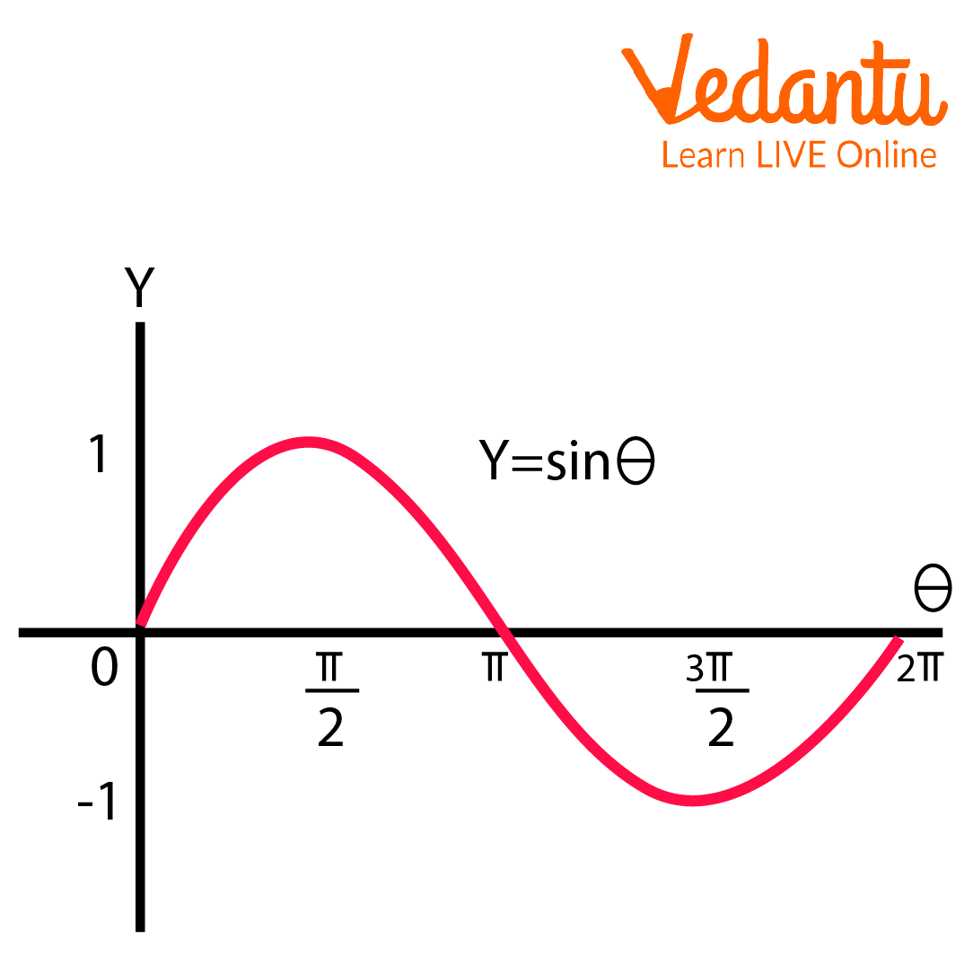
Sin function
Properties of Reduction
Reduction Formulas are used to evaluate higher order integrals that cannot be evaluated otherwise.
Reductions Formulas are applicable across a wide range of variables such as exponential, logarithmic, algebraic, trigonometric, etc.
Area Under the Curve
Solved Examples
1. Find the integral of \[\sin ^{5 x}\].
Ans:
Apply reduction formula:
$\Rightarrow-\dfrac{1}{5} \cdot \sin ^{4} x \cdot \cos x+\dfrac{4}{5} \int \sin ^{3} x \cdot d x \\$
$\Rightarrow-\dfrac{1}{5} \cdot \sin ^{4} x \cdot \cos x+\dfrac{4}{5}\left(\int \dfrac{(3 \sin x-\sin 3 x)}{4} \cdot d x\right) \\$
$\Rightarrow-\dfrac{1}{5} \cdot \sin ^{4} x \cdot \cos x+\dfrac{1}{5}\left(3 \int \sin x \cdot d x-\int \sin 3 x \cdot d x\right) \\$
$\Rightarrow-\dfrac{1}{5} \sin ^{4} x \cdot \cos x+\dfrac{1}{5}\left(-3 \cos x+\dfrac{\cos 3 x}{3}\right) \\$
$\Rightarrow-\dfrac{1}{5} \cdot \sin ^{4} x \cdot \cos x-\dfrac{3 \cos x}{5}+\dfrac{\cos 3 x}{15}$
Therefore, we have
$\Rightarrow \int \sin ^{5} x \cdot d x=-\dfrac{1}{5} \cdot \sin ^{4} x \cdot \cos x-\dfrac{3 \cos x}{5}+\dfrac{\cos 3 x}{15}$
2. Evaluate the integral of $x^{3} \log ^{2} x$.
Ans:
Applying the reduction formula:
$\int x^{n} \log ^{m} x \cdot d x=\dfrac{x^{n+1} \log ^{m} x}{n+1}-\dfrac{m}{n+1} \int x^{n} \log ^{m-1} x . \\$
$\int x^{3} \log ^{2} x \cdot d x=\dfrac{x^{4} \log ^{2} x}{4}-\dfrac{2}{4} \int x^{3} \log x \cdot d x \\$
$\Rightarrow \dfrac{x^{4} \log ^{2} x}{4}-\dfrac{1}{2}\left(\dfrac{x^{4} \log x}{4}-\dfrac{1}{4} \cdot \int x^{3} \cdot d x\right) \\$
$\Rightarrow \dfrac{x^{4} \log ^{2} x}{4}-\dfrac{x^{4} \log x}{8}+\dfrac{x^{4}}{32}+C$
Therefore, we have
$\Rightarrow \int x^{3} \log ^{2} x \cdot d x=\dfrac{x^{4} \log ^{2} x}{4}-\dfrac{x^{4} \log x}{8}+\dfrac{x^{4}}{32}+C$
3. Evaluate $\int_{0}^{2 a} x^{2} \sqrt{2 a x-x^{2}} d x$.
Ans:
So, $d x=-4 a \cos \theta \sin \theta d \theta$.
At $x=0,2 \operatorname{acos}^{2} \theta=0$ and so $\theta=\dfrac{\pi}{2}$.
When $x=2 a, 2 a \cos ^{2} \theta=2 a$ and so $\theta=0$.
Hence, we have
$\Rightarrow I=\int_{0}^{2 a} x^{2} \sqrt{2 a x-x^{2}} d x$
$\Rightarrow \int_{\dfrac{\pi}{2}}^{0} 4 a^{2} \cos ^{2} \theta \sqrt{4 a^{2} \cos ^{2} \theta-4 a^{2} \cos ^{4} \theta}(-4 a \cos \theta \sin \theta) d \theta$
$\Rightarrow \int_{0}^{\dfrac{\pi}{2}} 4 a^{2} \cos ^{2} \theta 2 a \cos \theta \sin \theta(4 a \cos \theta \sin \theta) d \theta$
$\Rightarrow 32 a^{4} \int_{0}^{\dfrac{\pi}{2}} \cos ^{4} \theta \sin ^{2} \theta d \theta$
$\Rightarrow 32 a^{4} \times \dfrac{1}{6} \times \dfrac{3}{4} \times \dfrac{1}{2} \times \dfrac{\pi}{2}$
$\Rightarrow \pi a^{4}$
Conclusion
In the article, we have discussed the detailed proof of Reduction Formulas and their applications. They are very helpful and reduce our computational work. So, reduction formulas are very important and can be derived using simple integration formulas; however, the proof is not important for us, so we need to remember all the formulas used to compute higher-order integrals.
Important Points to Remember
All the Reduction Formulas are important and are to be remembered.


FAQs on Reduction Theorem and Trigonometric Angle Reduction
1. What is the Reduction Theorem in linear algebra?
The Reduction Theorem states that any matrix can be reduced to a normal (canonical) form using a finite sequence of elementary row and column operations. In particular, every matrix is equivalent to a matrix of the form:
\( \begin{bmatrix} I_r & 0 \\ 0 & 0 \end{bmatrix} \)
where r is the rank of the matrix and I_r is the identity matrix of order r. This theorem is fundamental in finding the rank, solving systems of linear equations, and studying linear transformations.
2. What is the normal form of a matrix according to the Reduction Theorem?
The normal form of a matrix under the Reduction Theorem is \( \begin{bmatrix} I_r & 0 \\ 0 & 0 \end{bmatrix} \), where r is the rank of the matrix. This form is obtained by applying elementary row and column operations. The matrix contains:
- An identity matrix I_r in the top-left corner
- Zeros elsewhere
3. How do you find the rank of a matrix using the Reduction Theorem?
The rank of a matrix is the number of non-zero rows in its normal form obtained using the Reduction Theorem. To find it:
- Apply elementary row and column operations.
- Reduce the matrix to its normal form.
- Count the number of leading 1s (pivot positions).
4. What are elementary operations used in the Reduction Theorem?
The Reduction Theorem uses elementary row and column operations to simplify a matrix. These operations include:
- Interchanging two rows (or columns)
- Multiplying a row (or column) by a non-zero scalar
- Adding a multiple of one row (or column) to another
5. Can you give an example of the Reduction Theorem?
Yes, for example, consider the matrix:
\( A = \begin{bmatrix} 1 & 2 \\ 2 & 4 \end{bmatrix} \)
Apply row operations:
- R₂ → R₂ − 2R₁
\( \begin{bmatrix} 1 & 2 \\ 0 & 0 \end{bmatrix} \)
This is already in normal form with one pivot, so the rank = 1. This demonstrates the Reduction Theorem in action.
6. Why is the Reduction Theorem important?
The Reduction Theorem is important because it provides a systematic way to determine the rank, solve systems of linear equations, and analyze linear transformations. It helps in:
- Checking consistency of equations
- Finding inverse matrices (when rank equals order)
- Understanding linear independence
7. What is the difference between row echelon form and normal form in the Reduction Theorem?
Row echelon form is obtained using only row operations, while normal form in the Reduction Theorem uses both row and column operations. Key differences:
- Row echelon form: Staircase pattern with pivots
- Normal form: Reduced to \( \begin{bmatrix} I_r & 0 \\ 0 & 0 \end{bmatrix} \)
8. Does the Reduction Theorem change the determinant of a matrix?
Yes, elementary operations used in the Reduction Theorem can change the determinant value, but they do not change the rank. Specifically:
- Row interchange changes the sign of the determinant.
- Multiplying a row by k multiplies the determinant by k.
- Adding a multiple of one row to another does not change the determinant.
9. How is the Reduction Theorem used to solve linear systems?
The Reduction Theorem is used to solve linear systems by reducing the augmented matrix to normal or echelon form. Steps:
- Form the augmented matrix [A | B].
- Apply elementary row operations.
- Reduce to echelon or reduced form.
10. What is the connection between the Reduction Theorem and matrix equivalence?
The Reduction Theorem shows that two matrices are equivalent if one can be transformed into the other using elementary row and column operations. All matrices with the same rank r are equivalent to the same normal form:
\( \begin{bmatrix} I_r & 0 \\ 0 & 0 \end{bmatrix} \)
This establishes that rank completely determines matrix equivalence under these operations.