Final Value Theorem of Laplace Transform

The Final Value Theorem is a fundamental tool in a circuit system working. It is based on Laplace functions and their transformation. So, to understand the final theorem, we need to have some idea about Laplace transformations. In this article, we will be discussing the final value theorem in depth. We will also discuss the application of the final value theorem in circuit systems and how problems related to the theorem can be solved will also be discussed in this article. Below is the figure which shows the state for a function:

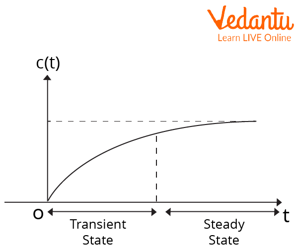
Steady-state Function

History of Pierre-Simon Laplace

Pierre-Simon Laplace

• Name: Pierre-Simon Laplace

• Born: 23 March 1749

• Died: 5 March 1827

• Field: Mathematics

• Nationality: French

Statement of the Final Value Theorem

The final value theorem states that if $x$ is any function of $t$ and Laplace transformation of $x$ is denoted as X(s), i.e., \[x(t) \underrightarrow{L T} X(s)\]

then,

$\mathop{\lim}\limits_{t \rightarrow \infty}x(t)=x(\infty)=\mathop{\lim}\limits_{s \rightarrow 0}sX(s)$

Here, LT represents Laplace Transformation.

Proof of the Final Value Theorem

From the definition of the unilateral Laplace transform, we have

$L[x(t)]=X(s)=\int_{0}^{\infty} x(t) e^{-s t} d t$

Taking differentiation with respect to time on both sides, we get $L\left[\dfrac{d x(t)}{d t}\right]=\int_{0}^{\infty} \dfrac{d x(t)}{d t} e^{-s t} d t$

Now, by the time differentiation property, i.e., $\dfrac{d x(t)}{d t} \underrightarrow{L T}\:s X(s)-x\left(0^{-}\right)$ of Laplace transform, we have

$L\left[\dfrac{d x(t)}{d t}\right]=\int_{0}^{\infty} \dfrac{d x(t)}{d t} e^{-s t} d t=s X(s)-x\left(0^{-}\right)$

By taking the $\mathop{\lim}\limits_{s \rightarrow 0}$ on both sides of the above expression, we get

$\mathop{\lim}\limits_{s\to0}[\int_{0}^{\infty}\dfrac{\text{d}x(t)}{\text{d}t}e^{-st}dt]=\mathop {\lim }\limits_{s \to0}[sX(s)-x(0^{-})]$

$\Rightarrow \int_{0}^{\infty} \dfrac{d x(t)}{d t} d t=\mathop{\lim}\limits _{s \rightarrow 0}\left[s X(s)-x\left(0^{-}\right)\right]$

$\Rightarrow[x(t)]_{0}^{\infty}=\mathop{\lim}\limits _{s \rightarrow 0}\left[s X(s)-x\left(0^{-}\right)\right]$

$\Rightarrow x(\infty)-x\left(0^{-}\right)=\mathop{\lim}\limits_{s \rightarrow 0}\left[s X(s)-x\left(0^{-}\right)\right]$

$\Rightarrow x(\infty)=\mathop{\lim}\limits_{s \rightarrow 0} s X(s)$

Therefore, we have

$\mathop{\lim}\limits_{t \rightarrow \infty} x(t)=x(\infty)=\mathop{\lim}\limits_{s \rightarrow 0} s X(s)$

Limitations of the Final Value Theorem

• The Final Value theorem does not apply when the Laplace transform has imaginary but non-zero poles as the limit of time response does not exist.

• The Final Value theorem does not apply when the pole is in the right half plane.

Applications of the Final Value Theorem

• The Final Value theorem has wide application in electronic devices or circuits.

• The Final Value theorem is used to find the steady or transient state of a function.

• The Final Value theorem is used to find the transient state gain of a wash-out function.

Solved Examples

1. What is the steady state value of f(t), if it is known that $F(s)=\dfrac{2}{s(s+1)(s+2)(s+3)}$.

Ans: From the equation of $F(s)$, we can infer that a simple pole is at the origin and all other poles are having negative real parts.

$\therefore f(\infty)=\mathop{\lim}\limits_{s \rightarrow 0} s F(s) $

$\Rightarrow f(\infty)=\mathop{\lim}\limits_{s \rightarrow 0} \dfrac{2 s}{s(s+1)(s+2)(s+3)} $

$\Rightarrow f(\infty)=\dfrac{2}{(s+1)(s+2)(s+3)} $

$\Rightarrow f(\infty)=\dfrac{2}{6} $

$\Rightarrow f(\infty)=\dfrac{1}{3}$

2. What will be the inverse Laplace transform of \[F(s)=\dfrac{2}{s^{2}+3 s+2}\]?

Ans: $s^{2}+3 s+2=(s+2)(s+1)$

Now, $F(s)=\dfrac{A}{(s+2)}+\dfrac{B}{(s+1)}$

Hence, $A=\left.(s+2) F(s)\right|_{s=-2}$

$\Rightarrow A=\left.\dfrac{2}{s+1}\right|_{s=-2}$

$\Rightarrow A=-2$

And, $B=\left.(s+1) F(s)\right|_{s=-1}$

$\Rightarrow B=\left.\dfrac{2}{s+2}\right|_{s=-1}$

$\Rightarrow B=2\\$

$\therefore F(s)=\dfrac{-2}{(s+2)}+\dfrac{2}{(s+1)} $

$\therefore F(t)=L^{-1}\{F(s)\} $

$\Rightarrow F(t)=-2 e^{-2 t}+2 e^{-t} \text { for } t \geq 0$

3. What will be the inverse Laplace transform of $F(s)=\dfrac{2}{s+c} e^{-b s}$?

Ans: $\text { Let } G(s)=\dfrac{2}{s+c} $

$\text { Or, } G(t)=L^{-1}\{G(s)\} $

$\Rightarrow G(t)=2 e^{-c} $

$\therefore F(t)=L^{-1}\left\{G(s) e^{-b s}\right\} $

$\Rightarrow F(t)=2 e^{-k(t-b)} u(t-b)$

Important Formulas to Remember

• If $x(t)\:\underrightarrow{L T}\:X(s)$,

Then $\mathop{\lim}\limits_{t \rightarrow \infty} x(t)=x(\infty)=\mathop{\lim}\limits_{s \rightarrow 0} s X(s)$

• Laplace transformation: $L[f(t)]=F(s)=\int_{0}^{\infty} f(t) e^{-s t} d t$

Important Points to Remember

• Laplace transformation is an essential tool to learn the final value theorem.

• Circuit Diagrams and electric circuits are based on the application of the final value theorem.

Conclusion

The Final Value Theorem has a wide range of applications in daily life and it is a fundamental tool for functional analysis and electrical circuits. In the above article, we have discussed the Final Value theorem in brief, and the limitations of the theorem are also discussed. So, in short, we can say that the Final Value theorem forms a vital component of our life and makes our day-to-day work easy.