Question

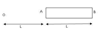
A charge \[Q\] is uniformly distributed over a long rod AB of length \[L\] as shown in the figure. The electric potential at the point O lying at distance \[L\] from the end A is

\[\dfrac{Q}{{8\pi {\varepsilon _0}L}}\]
\[\dfrac{{3Q}}{{4\pi {\varepsilon _0}L}}\]
\[\dfrac{Q}{{4\pi {\varepsilon _0}L\ln 2}}\]
\[\dfrac{{Q\ln 2}}{{4\pi {\varepsilon _0}L}}\]

Answer 1

Hint: We are asked to find the potential at point O due to rod AB. First find the line charge density of the rod. Take a small element from the rod and find its potential at the given point. Use this potential due to an element of rod AB to find the potential due to the whole rod AB at the given point.

Complete step by step answer:
Given, the length of the rod AB is \[L\] and charge \[Q\] is uniformly distributed over the rod AB.
Let \[\lambda \] be the line charge density, line charge density can be written as,
\[\lambda = \dfrac{{{\text{Charge}}\,}}{{{\text{Length}}}}\]
\[ \Rightarrow \lambda = \dfrac{Q}{L}\]
First, we take a small element \[dx\] of the rod AB at a distance \[x\] from point O.

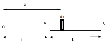
Self-made diagram

Potential at O due to the element \[dx\] can be written as,
\[dV = \dfrac{1}{{4\pi {\varepsilon _0}}}\dfrac{Q}{x}\] (i)
For length \[L\], line charge density is, \[\lambda = \dfrac{Q}{L}\] and for \[dx\] length line charge density will be
\[\lambda = \dfrac{Q}{{dx}}\]
\[ \Rightarrow Q = \lambda dx\]
Now, substituting this value of \[Q\] in equation (i), we get
\[dV = \dfrac{1}{{4\pi {\varepsilon _0}}}\dfrac{{\lambda dx}}{x}\] (ii)
This is the potential due to a small element \[dx\]. To find the potential due to the whole rod AB we integrate equation (iii) from \[L\] to \[2L\]. We take \[L\] to \[2L\]because the distance between point O and one end of the rod is \[2L\] and the other end is \[L\] .
\[\therefore V = \int\limits_L^{2L} {\dfrac{1}{{4\pi {\varepsilon _0}}}\dfrac{{\lambda dx}}{x}} \\\
   \Rightarrow V = \dfrac{\lambda }{{4\pi {\varepsilon _0}}}\int\limits_L^{2L} {\dfrac{{dx}}{x}} \\\
   \Rightarrow V = \dfrac{\lambda }{{4\pi {\varepsilon _0}}}\left[ {\ln x} \right]_L^{2L} \\\]
\[\Rightarrow V = \dfrac{\lambda }{{4\pi {\varepsilon _0}}}\left[ {\ln (2L) - \ln (L)} \right] \\\
   \Rightarrow V = \dfrac{\lambda }{{4\pi {\varepsilon _0}}}\ln \dfrac{{2L}}{L} \\\
   \Rightarrow V = \dfrac{\lambda }{{4\pi {\varepsilon _0}}}\ln 2 \\\]
For, whole length \[L\] the line charge density is \[\lambda = \dfrac{Q}{L}\]. So, the potential will be
\[V = \dfrac{{Q\ln 2}}{{4\pi {\varepsilon _0}L}}\]
Therefore, the potential at point O at distance \[L\] from one end of rod AB is \[V = \dfrac{{Q\ln 2}}{{4\pi {\varepsilon _0}L}}\]
\[V = \dfrac{{Q\ln 2}}{{4\pi {\varepsilon _0}L}}\]

So, the correct answer is “Option D”.

Note:
In problems where potential due to the whole object is difficult to find, always take a small element of the object and find its potential at the given point and integrate this value to find the potential of the object at the given point. Here, the charge was uniformly distributed but if the charge is non uniform then we would need to find their dependence on length.