Question

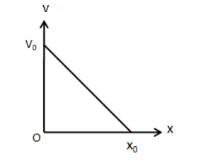
The velocity-displacement graph of a particle is shown in figure.
a) Write the relation between v and x.
b) Obtain the relation between acceleration and displacement and plot it.

Answer 1

Hint:Express the angle made by the straight line with the horizontal axis. Then assume the position of the particle at any point of the straight line and then express the angle made by this straight line with the horizontal axis. Comparing the two equations, we will get the relation between v and x. The derivative of velocity with respect to time is the acceleration of the particle.

Complete step by step answer:
(a) We have given the initial velocity \[{v_0}\] and displacement \[{x_0}\] at time \[t = 0\]. We can redraw the above figure as,

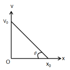
From the above figure, we can express \[\tan \theta \] as,
\[\tan \theta = \dfrac{{{v_0}}}{{{x_0}}}\] …… (1)
Now, we assume at any instant of time, the particle has velocity v and displacement x. The position of the particle is shown by the point A in the following figure.

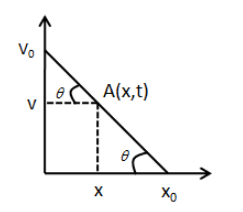
We can express \[\tan \theta \] as,
\[\tan \theta = \dfrac{{{v_0} - v}}{x}\] …… (2)
From equation (1) and (2), we can write,
\[\dfrac{{{v_0}}}{{{x_0}}} = \dfrac{{{v_0} - v}}{x}\]
\[ \Rightarrow {v_0}x = {v_0}{x_0} - v{x_0}\]
\[ \Rightarrow v = \dfrac{1}{{{x_0}}}\left( {{v_0}{x_0} - {v_0}x} \right)\]
\[ \therefore v = - \dfrac{{{v_0}}}{{{x_0}}}x + {v_0}\] …… (3)
This is the relation between v and x.

(b) We know that the acceleration is the derivative of velocity of the particle. Therefore, we can write.
\[a = \dfrac{{dv}}{{dt}}\]
We have the expression for velocity obtained in part (a) of the solution. Therefore, the acceleration of the particle is,
\[a = \dfrac{d}{{dt}}\left( { - \dfrac{{{v_0}}}{{{x_0}}}x + {v_0}} \right)\]
\[ \Rightarrow a = - \dfrac{{{v_0}}}{{{x_0}}}\dfrac{{dx}}{{dt}} + \dfrac{d}{{dt}}\left( {{v_0}} \right)\]
\[ \Rightarrow a = - \dfrac{{{v_0}}}{{{x_0}}}v\]
Using equation (3), we can rewrite the above equation as,
\[a = - \dfrac{{{v_0}}}{{{x_0}}}\left( { - \dfrac{{{v_0}}}{{{x_0}}}x + {v_0}} \right)\]
\[ \therefore a = \dfrac{{v_0^2}}{{x_0^2}}x - \dfrac{{v_0^2}}{{{x_0}}}\]
From the above expression, if the displacement of the particle x is zero. Then the acceleration of the particle is \[ - \dfrac{{v_0^2}}{{{x_0}}}\]. Also, the acceleration of the particle increases linearly with respect to the position of the particle. Therefore, we can plot the graph of acceleration and displacement as,

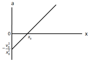
The acceleration is zero when the displacement \[x = {x_0}\] .

Note: In equation (1) and (2), the angle \[\theta \] is the same since it is the angle made by the same line with the horizontal axis. Always remember, the derivative of displacement with respect to time is the velocity and the derivative of velocity with respect to time is the acceleration. In the acceleration-displacement plot, the acceleration becomes zero at initial position \[{x_0}\] which can be found by assuming \[\dfrac{{v_0^2}}{{x_0^2}}x = \dfrac{{v_0^2}}{{{x_0}}}\] and solving for x.